Software is notorious for frequent and unanticipated changes. Websites appear, disappear, and are redesigned frequently. Features appear and disappear even in mature software like email clients, word processors and spreadsheets. R is no different. Here are a few changes that have occurred in the last few years that are particularly relevant to our course.
The “pipe” feature has become part of R (as of version 4.1), but it looks different than the old pipe and works a little bit differently. I don’t think this difference will affect the examples in this course very much. I have changed to the new pipe (|>) most places in the examples, but the old pipe (%>%) probably still appears in some places.
GitHub authentication has changed; passwords are no longer allowed from R (or anywhere except the website). I have revised and simplified the instructions for using GitHub. This is a technical subject that can be difficult for beginners to master—give yourself some time to fully understand how git and github work.
Data sources and external links disappear and change frequently. I think I have checked them all. If you see problems, let me know!
Overview
R is a big software package that has developed over decades of use. It has millions of regular users across many disciplines in teaching, academic research and professional applications. It’s a computer programming language, and a tool for accessing thousands of data analysis tools, and a great interactive environment for exploring, analyzing, and visualizing data. You won’t learn it all.
The approach in this course is to teach you how to use R in a particular style, with an emphasis on the ggplot and tidyverse packages. The R markdown documents we write balance interactive use while documenting the sequence of steps used in any analysis. I have omitted a lot of details that might be called “fundamentals” and instead focused on getting work done quickly. In this lesson I fill in some of the gaps. My reasoning is that most students want to learn a tool before you spend too much time on details, so this course emphasizes what you can do with R. On the other hand, I hope you will use R for a long time on many projects, and once you reach the point you know you will do that, you should start developing a solid mental model of how R works so that you can build robust understandings of how to accomplish tasks with R and get beyond copy, paste, search, and experiment. Without these fundamentals, its easy to make up incorrect ideas about why and how R works and then get really confused and frustrated.
A simple introduction to the basics of R appears in Healy Appendix. A different approach is taken in the R for Data Science book, which introduces the basics of many topics, such as tibbles, strings, factors and dates, functions and vectors together with their applications one chapter at a time.
What kinds of data structures does R use?
R has many basic types: logical, numeric (double), character, factor. Any combination of these types can be combined into lists. Elements of lists can be named so that they work like dictionaries. Vectors, matrices, and higher dimensional arrays are all composed of the same type of data, usually numeric, factor, or logical.
Lists are a very powerful type because they can be given attributes that identify them as special structures with particular interpetations. The most common special list is a data frame, data table or tibble. (The tibble is a refined kind of data frame.) You probably think of a tibble as a matrix where each column can be of a different type. How is this accomplished? It’s a list of vectors. Each vector corresponds to a column or variable in the data frame with its own name and data type.
Here are some R commands you can use to decode the structure of any object you have in your workspace. I’ll demonstrate on the diamonds tibble. As always, experiment with these commands by trying them on other objects such as cars (a data frame).
When R was young, there was one way to organize data into the tables we are using throughout this course: the data frame. This data structure is made from a list of vectors; each column is an entry in the list and all the data in each list (column) must be of the same type. Over time, people wanted to add new features to data tables, but existing code made this difficult. So two new kinds of data frames were created.
A tibble is a data frame, but it has some extra features. Most notably the way it is displayed in R has been improved. Only a few rows and columns are shown (unless you ask for more) with the rest of the information provided as a summary. Tibbles are widely used by the tidyverse packages.
A data table is a kind of data frame where all the code has been written with the goal of increasing calculation speed. Some of the methods for manipulating data tables are quite different from what we have learned in this course; some of the examples from R4DS chapter on data transformations are demonstrated here.
What is the difference between strings and factors?
A string is just a sequence of text, enclosed by single or double quotation marks. You can display strings, and search for text, and do other text-type things with them, but you can’t (of course) do calculations with them.
You can convert a vector of strings into a vector of factors. This assigns an integer to each different element in the vector. Why would you do this? The numbers can be assigned to give a particular order to the factors (strings) that is different from alphabetical. The factors can be used in statistical models as though they are numbers, as though they were the indexes you use on a variable in math class (e.g., \(x_1, x_2, \dots\)).
[1] Apple   Bananna Cat     Apple   Orange
Levels: Apple Bananna Cat Orange
The forcats package has lots of great functions for working with factors which can help you control how your plots are drawn. That’s the main use we will have for them in this course.
What’s the pipe?
The pipe %>% is a way to write function composition. In our data analysis we build up calculations from lots of different functions such as select, group_by, arrange, filter, summarize, distinct and many more described in R for Data Science. Each function starts with a tibble, does something to it, and produces a revised tibble. It’s very natural to develop a complex series of calculations like a recipe in a cookbook. (Sometimes these recipes are called pipelines!) Before pipes were invented there were basically two options; write the functions down in reverse order, or create lots of temporary variables to store the intermediate results and then discard them. Pipelines are easier to write and easier to read. Here’s an example of the three styles, based on a simple analysis of the diamonds data.
# A tibble: 7 × 2
  color mean_price
  <ord>      <dbl>
1 D          2629.
2 E          2598.
3 F          3375.
4 G          3721.
5 H          3889.
6 I          4452.
7 J          4918.
Which do you think is easier to understand? What if the pipline was longer? Or shorter?
Note: as of late 2020, a new kind of pipe is becoming part of R. It looks like this |> and works a bit like the existing pipe we use but has some differences. It’s not in this course at all yet since the official release of R doesn’t have it. This is another example of how R (and all computer systems) change over time. These sorts of big changes are very rare with R because so many people use it for so many purposes.
Why does ggplot use +?
When we make plots with ggplot we do something very similar – we start with a tibble or data frame, but then we make a plot, and then modify it step by step, setting geometries, adding more data, creating facets, setting scales, altering the theme. This seems a lot like a pipeline. Why do we use + to connect different ggplot2 commands?
Simple. The developer didn’t know about the pipe operator in R when ggplot was developed. Adding a feature to a plot seemed like a “plus” operation, so that was chosen. The developer says if he was starting over today, ggplot would use pipes, but its not practical to change at this point. Too many people use it with the +. Some people think of functions as verbs and ggplot commands as nouns, and justify the difference that way. Software development is a complicated human activity that takes place over time and develops quirks and lore.
What are packages? What’s the difference between installing one and using one? Why is R organized this way?
There are thousands of R packages. So many that it seems you are always needing to install a new one. Worse, sometimes you want a function, but you can’t remember which package it’s installed in – so then you can’t use it. (There is a solution to this: use the double ?? followed by the fuction name in the console to search for a function across all packages available on your computer.) Why this complication?
There are several reasons.
New packages are developed frequently, by different people. And some packages get abandoned too. Packages create modularity that makes it easier to test and fix problems with packages across different groups of developers.
The library command tells R you want to use a particular package in your current session. Not loading all packages can save time, computer resources, and avoid name collisions (see below).
Most people only use a small fraction of all the packages available – you simply don’t need to install them all.
Two packages can use the same name for a different function or different dataset. If there were no packages, everyone using R would have to coordinate the naming of everything across all the packages. An impossible task. Sometimes when you load a package with library you’ll get a message that an existing function has been redefined (or masked) by this new package. You can always add the package name and two colons, dplyr::filter for example, to refer to a function in a particular package.
Why are there so many kinds of “equals signs”?
There are many different concepts behind the humble equals sign used in mathematics. In R we use different symbols: =, ==, <- and even some special functions like all.equal and near. Even with all these differences = can mean different things in different contexts, and there is a special version of <- written in the other way: ->. The pipe adds its own twist, you can write %<>% as a combined assignment operator and pipe.
So what does each mean?
a <- b means assign the name a to the object b. (You can use = for this, but I encourage you not to.)
a == b is a comparison between a and b with the result TRUE if they are the same and otherwise FALSE. (The notion of “same” in computing is surprisingly complicated, but for basic types, in particular strings, this is fairly straightforward.)
a = b is used when naming elements of a list or arguments to a function, for example ggplot(mapping = aes(...)) or list(a= "apple", b="bananna").
near(1.25, 1.253, tol = 0.01) in the dplyr package is used to compare numbers to see if they are close together.
The waldo package has functions for testing equality of data frames and showing differences.
Numbers
R has several different kinds of ways of storing numbers that are encountered in data analysis and statistics. Two are familiar: integers and numbers with a decimal point (called floating point numbers). You can create, test, and convert numbers to integers using the functions integer, is.integer, and as.integer:
There are some special numbers: positive and negative infinity, not a number (NaN) and a missing number (or other kind of data) NA. You get plus or minus infinity when you divide a non-zero number by 0 and NaN is the result when you divide 0 by 0.
5/0
[1] Inf
-2/0
[1] -Inf
0/0
[1] NaN
NA works to protect you from getting numeric answers when you are missing data:
as.numeric("three")# get NA instead of an error, which can be handy or annoying
Warning: NAs introduced by coercion
[1] NA
What’s a function?
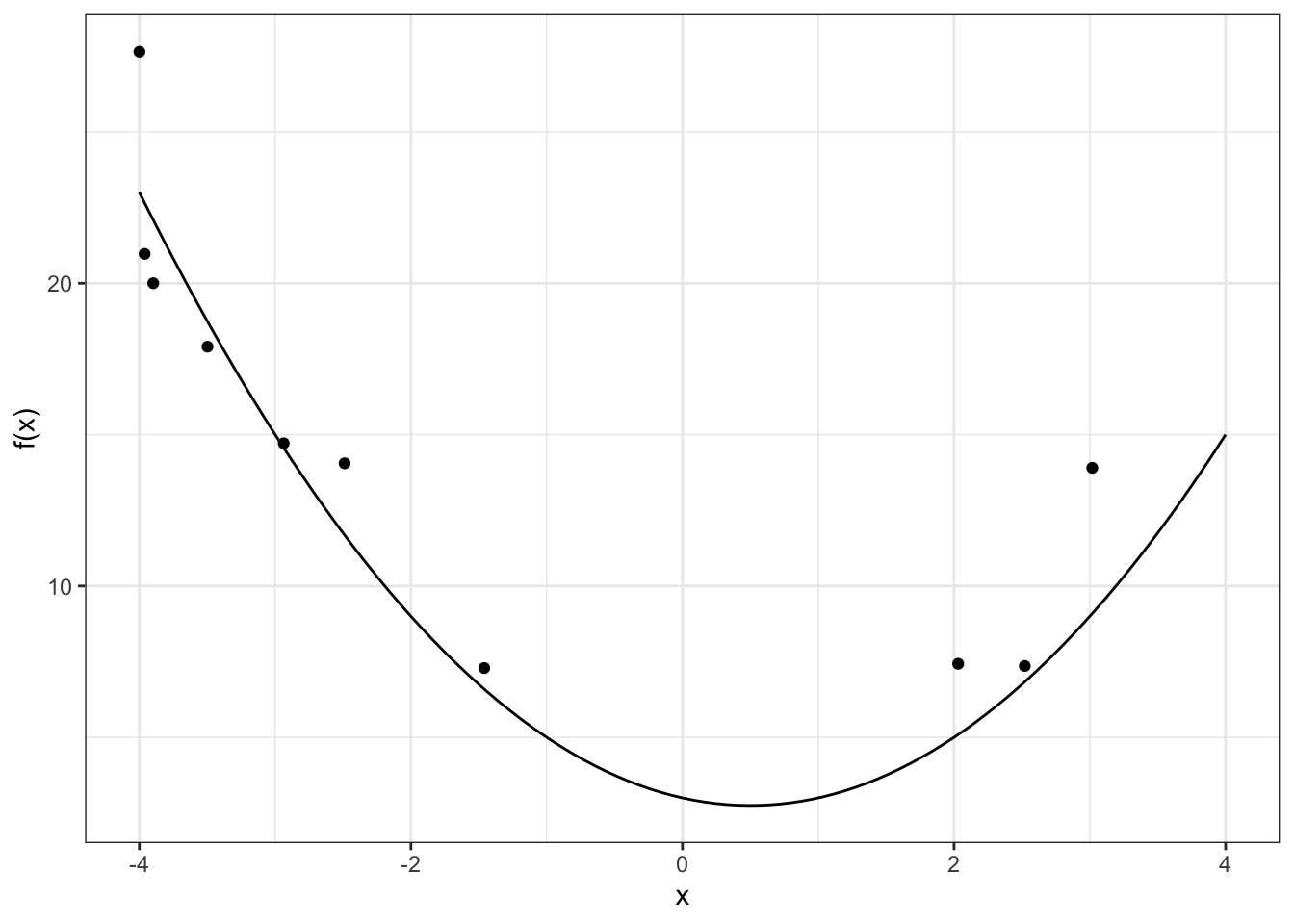
We’ll use the same definition offered in math class: a function is a rule that maps items in one set to items in another set. For example \(f(x) = x^2 - x + 3\). But R works with a lot more than numbers, so its functions do too.
All the code we have used with R in this course is built up from functions: library, ggplot, aes, geom_point, lm, tidy, summarize, unite, mean, sd, and the list goes on and on.
We can write our own functions too. This is handy in plotting, for example.
f<-function(x)x^2-x+3tibble(x =runif(10, -4, 4), y =rnorm(10, f(x), 3))|>ggplot()+geom_function(fun =f)+geom_point(aes(x, y))+theme_bw()+labs(x ="x", y ="f(x)")+xlim(-4, 4)
We have been using a consistent style of programming with R in this course. Wherever possible we use functions from the tidyverse package that accept tables (tibbles) as their first input and output tibbles when it makes sense to do so. (Plots are not tibbles for example, so ggplot doesn’t make them. But the result of using tidy on a linear regression model is a tibble.) Functions are connected together with the pipe (|> or %>%) to achieve a particular style of easy to read code and to avoid creating new temporary variables that don’t help with understanding the computation very much. This style of computing works very well in conjunction with the grammar of graphics style of plotting data.
There are lots of other ways to write code. One is known as base R. Another is based on tables, but using something called a data.table which is optimized for speed and a certain kind of concise notation. (Here is a concise introduction to some key concepts.)
Computing notes
There are thousands of different programming languages. Why? Partly different ideas have arisen over time. Sometimes, languages have been created for particular problems. But most often, languages are created to enable a new kind of interaction between programmer and computer. Over time, as computing power increases and the kinds of problems solved by computer change, new opportunities and new needs arise and new languages are developed.
What are some of the constraints and trade-offs when using a computer? The three most important are * the amount of storage required to solve a problem, * the number of computations to solve a problem, and * the amount of human time required to design and implement a solution.
Many programming languages prioritize the first two. The trade-off between the first two is a classic idea in computer science. You can see how it arises from a simple example. Suppose you know you need the approximate result of some complex mathematical computation. You can either perform the calcuation when you need it (which takes time), or you can compute a table of possible computations in advance (which takes storage) and lookup the result when you need it. This is the idea behind statistical tables in the back of statistics textbooks – the calculations are hard, but a good enough table fits on a page or two.
The designers of the R language and packages often prioritize minimizing the amount of time required for a human to design and code the solution to a problem. To do this well, the designers needed to give you flexible and powerful tools (functions). The flexibility of the functions means that they are not always optimized to use the least storage or time.
Powerful tools require significant study to learn how to use them effectively. The examples in this course are selected to convince you that that investment is worth your time. There are also many specialized packages of functions, each created to make a certain type of problem easier or faster to solve. This is now a feature of all programming domains, which have specialized tools for different operating systems, the web, or particular problem domains like databases, machine learningm or statistical data analysis. Each of these requires effort to learn, but a helpful insight comes from the early design of graphical user interfaces – if tools made by different programmers have enough in common and adhere to conventions, then the burden on the programmer and user is greatly reduced.
There are many other optimizations and trade-offs in computing. For example, numerical computations sometimes are done in a different order compared to the way you would do them in math class as a result of numerical approximations made by computers.
Even within the R system there are many different styles of programming and problem solving. In this course I emphasize one particular style, now known popularly as the tidyverse. This approach organizes data and results in tables (called tibbles) as much as possible and encourages you to build larger solutions from composing powerful functions together (like th dplyr package). As a result in this course a hidden message throughout most lessons is how to organize your data and results and how to use a small set of powerful functions to solve a large set of general problems.
Many other computing systems would work well for this course. Among programmers, a very popular choice is python, which shares a lot in common with R with many add-on packages providing similar functions. As a simplification, python use tends to be favoured by people developing software to solve a particular problem, while R tends to be favoured by people who want to interactively explore their data analysis options and need to develop custom analyses for each problem they encounter. Python and R have both existed since before the year 2000, but the styles of data analysis and problem solving possible with each has grown and converged together considerably in recent years.