gapminder |>
  filter(year == 2007) |>
  ggplot(aes(y=lifeExp,
             x=gdpPercap)) +
geom_point() 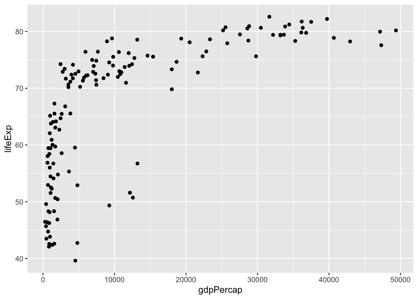
In this lesson we will find a visualization and try to reconstruct it using R.
A reasonable challenge is to redraw a version of the textbook cover for STAT 1060 (De Veaux et al. 2018) using the gapminder data.

Get the gapminder data, take the last year’s data (2007) and make a scatter plot:
The last year with data is 2007, so let’s take those data and make a scatterplot.
gapminder |>
filter(year == 2007) |>
ggplot(aes(y=lifeExp,
x=gdpPercap)) +
geom_point()
Change the x-axis to have a log scale. We can even use the log-2 scale.
Here’s a version with the abbreviated labels (16k) used on the cover, but avoiding the mistake of labelling 64k as 128k (neither appear on our graph).
We should clean up the axis names:
gapminder |> filter(year == 2007) |>
  ggplot(aes(y=lifeExp, x=gdpPercap)) +
  geom_point() +
  scale_x_continuous(trans = "log2") +
  xlab("Income per person, GCP/capita in $/year adjusted for inflation and prices") +
  ylab("") +
ggtitle("Life Expectancy (2007)") 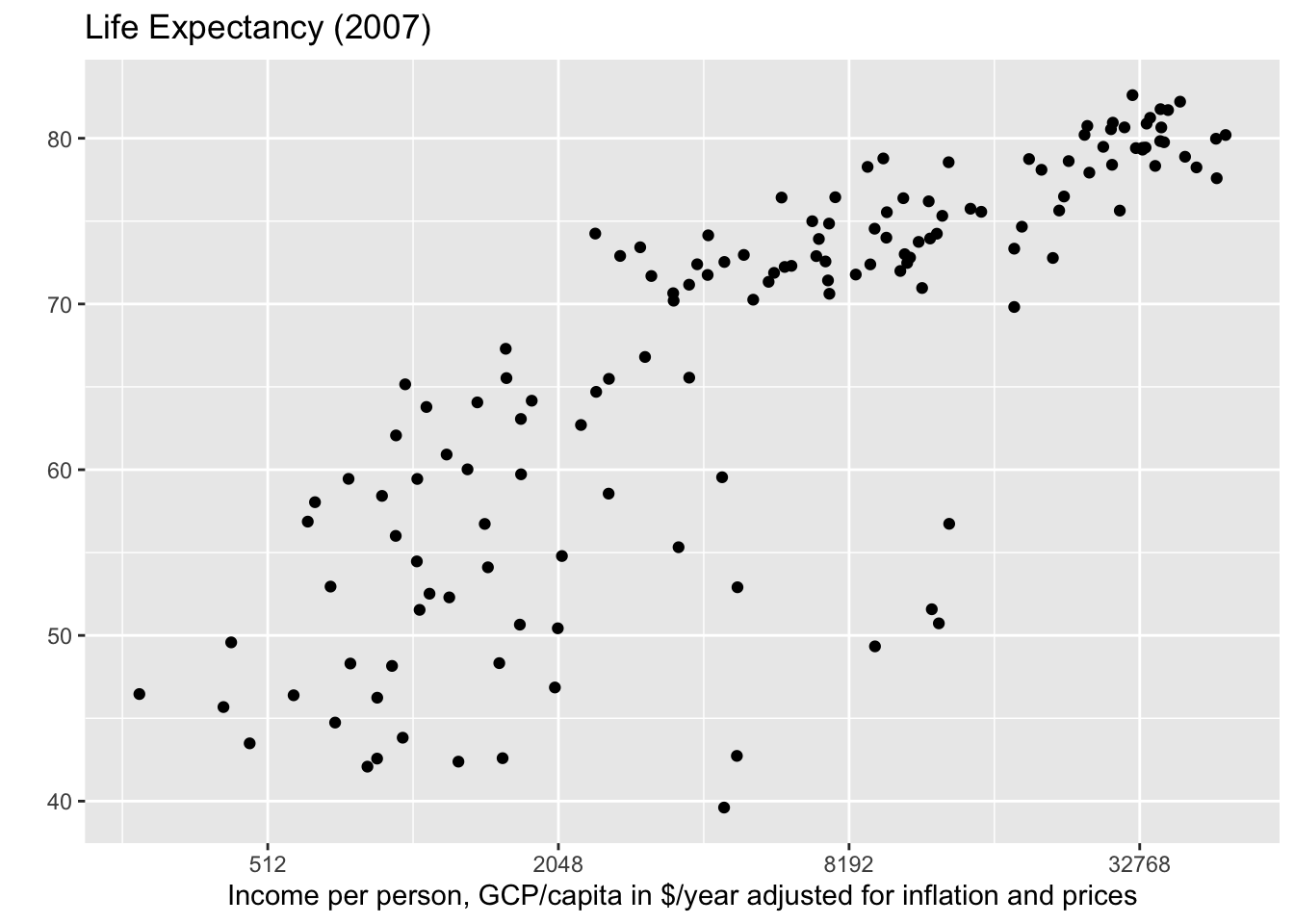
First colour from the continent name:
gapminder |> filter(year == 2007) |>
  ggplot(aes(y=lifeExp, x=gdpPercap, color=continent)) +
  geom_point() +
 scale_x_continuous(trans = "log2") +
  xlab("Income per person, GCP/capita in $/year adjusted for inflation and prices") +
  ylab("") +
ggtitle("Life Expectancy (2007)") 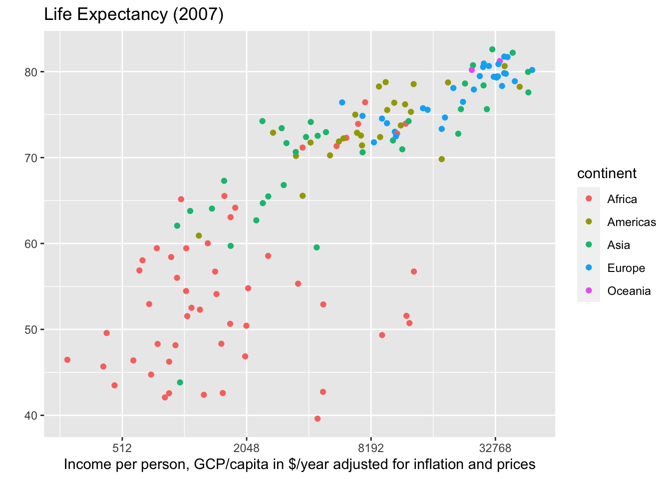
Add transparency, and outline around the points, match the colour to the book. Use population size to adjust the size of the dots.
gapminder |> filter(year == 2007) |>
  ggplot(aes(y=lifeExp, x=gdpPercap, color=continent, size = pop)) +
  geom_point(alpha=0.5) +
  geom_point(shape=1, color="black") +
  scale_x_continuous(trans = "log2") +
  xlab("Income per person, GCP/capita in $/year adjusted for inflation and prices") +
  ylab("") +
  ggtitle("Life Expectancy (2007)") +
scale_color_manual(values = c("blue", "green", "pink", "yellow", "red")) 
Scale the points by setting a maximum size. Remove the legend.
gapminder |> filter(year == 2007) |>
  ggplot(aes(y=lifeExp, x=gdpPercap, color=continent, size=pop)) +
  geom_point(alpha=0.5) +
  geom_point(shape=1, color="black") +
  scale_x_continuous(trans = "log2") +
  xlab("Income per person, GCP/capita in $/year adjusted for inflation and prices") +
  ylab("") +
  ggtitle("Life Expectancy (2007)") +
  scale_color_manual(values = c("blue", "green", "pink", "yellow", "red")) +
  scale_size_area(max_size = 20) +
  theme(legend.position = "none")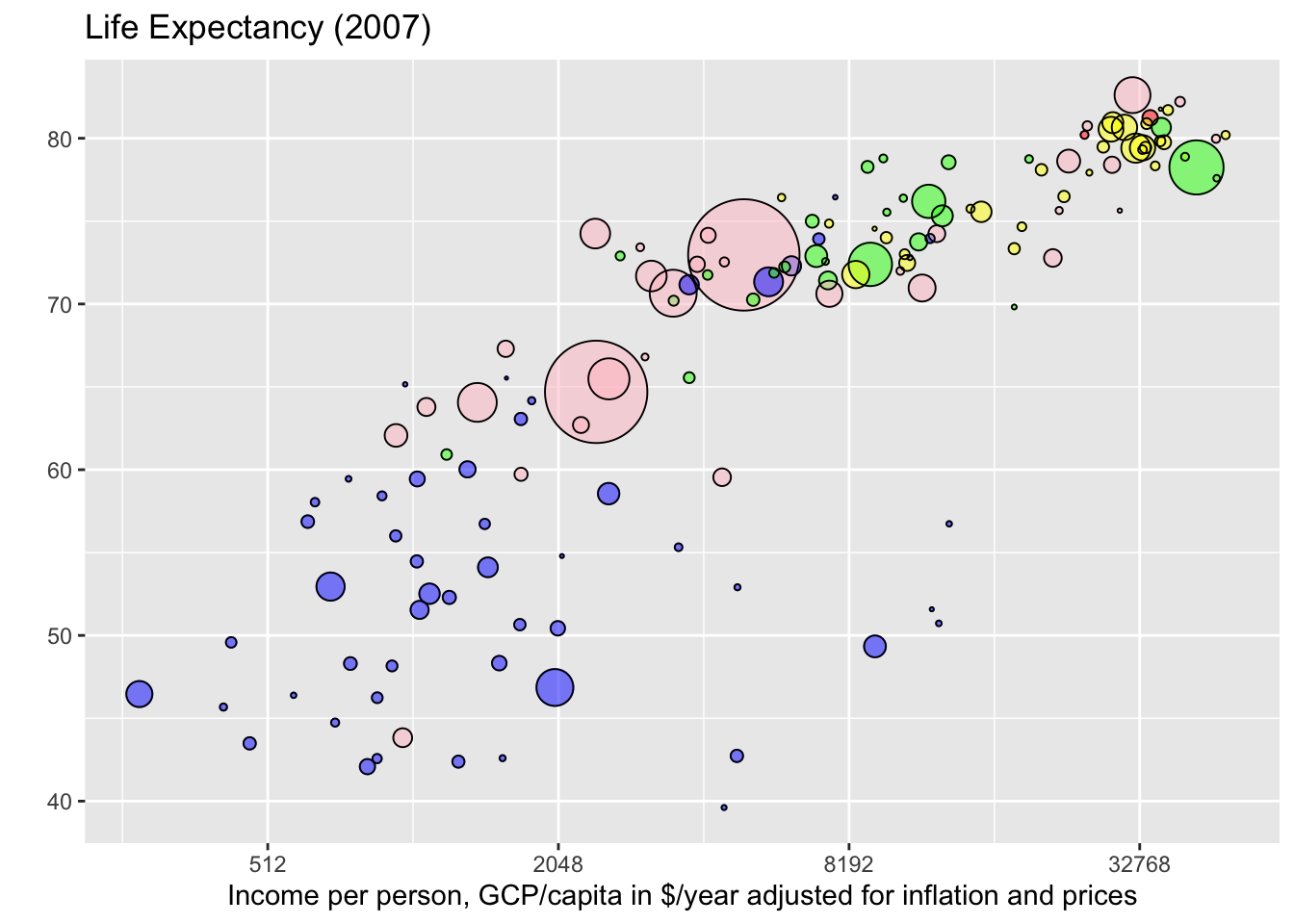
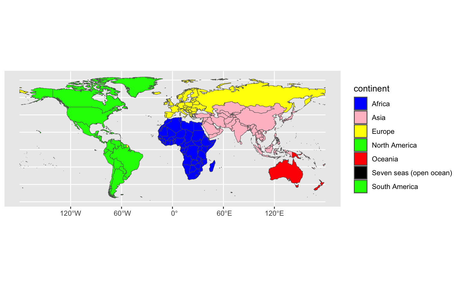
Make a map.
world <- ne_countries(scale='medium',
                      returnclass = 'sf')
world |>
  ggplot() +
  geom_sf(aes(fill=continent))
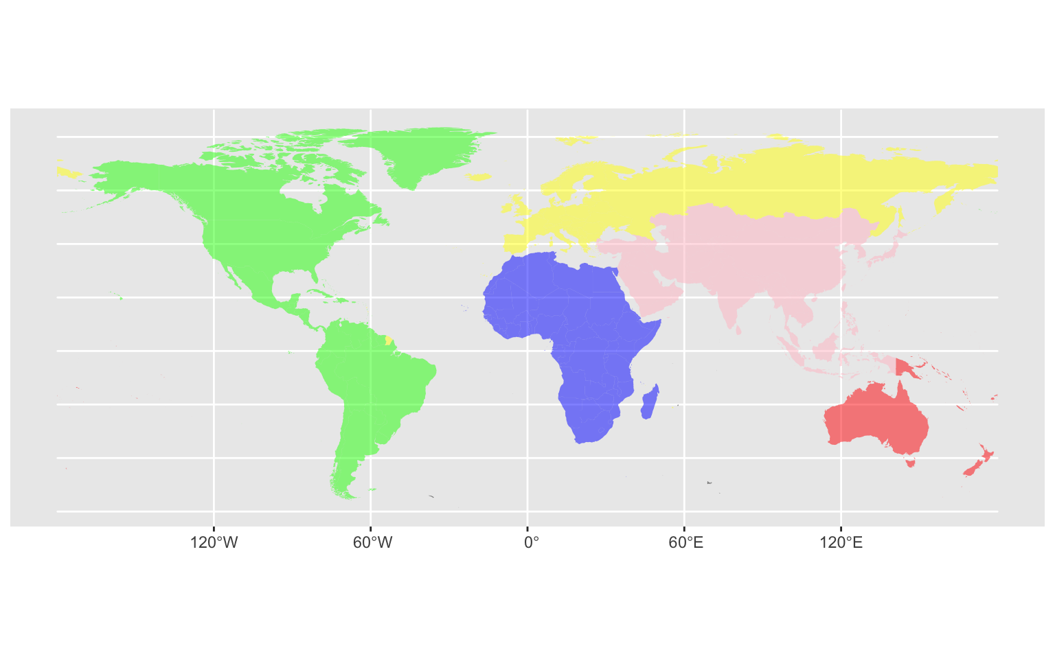
Remove Antarctica and match colours:
Remove outlines, add transparency, remove legend.
Remove the grid and background and axis labels:
world_map <- world |> filter(continent != "Antarctica") |>
  ggplot() + geom_sf(aes(fill=continent), color=NA, alpha=0.5) +
    scale_fill_manual(values = c("blue", "pink", "yellow","green", "red", "black", "green" )) +
    theme_bw() + theme(legend.position = "none", panel.border=element_rect(linetype=0),
                     panel.grid = element_line(color=NA),
                     panel.background = element_rect(fill=NA),
                     plot.background = element_rect(fill=NA),
                     axis.text.x = element_text(color=NA),
                     axis.ticks.length =  unit(0, "cm"))
world_map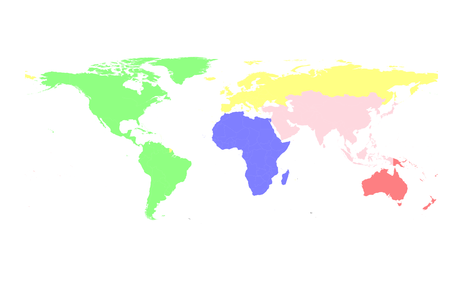
gapminder |> filter(year == 2007) |>
  ggplot(aes(y=lifeExp, x=gdpPercap, color=continent, size=pop)) +
  geom_point(alpha=0.5) +
  geom_point(shape=1, color="black") +
  geom_label_repel(aes(label=country), data = gapminder |> filter(year ==2007, country=="Canada"), color="black", fill="green",
                   segment.size=1, segment.color="green", box.padding=3) +
  xlab("Income per person, GCP/capita in $/year adjusted for inflation and prices") +
  ylab("") +
  ggtitle("Life Expectancy (2007)") +
  scale_color_manual(values = c("blue", "green", "pink", "yellow", "red")) +
  scale_size_area(max_size = 20) +
  annotation_custom(grob=ggplotGrob(world_map), xmin=12.3, ymin=35, ymax=50 ) +
  scale_x_continuous(trans = "log2",
                     labels = c("250", "500", "1000", "2000", "4000", "8000", "16k", "32k", "64k"),
                     breaks = c(250, 500, 1000, 2000, 4000, 8000, 16000, 32000, 64000)) +
  theme(legend.position = "none")  -> final_plot
final_plot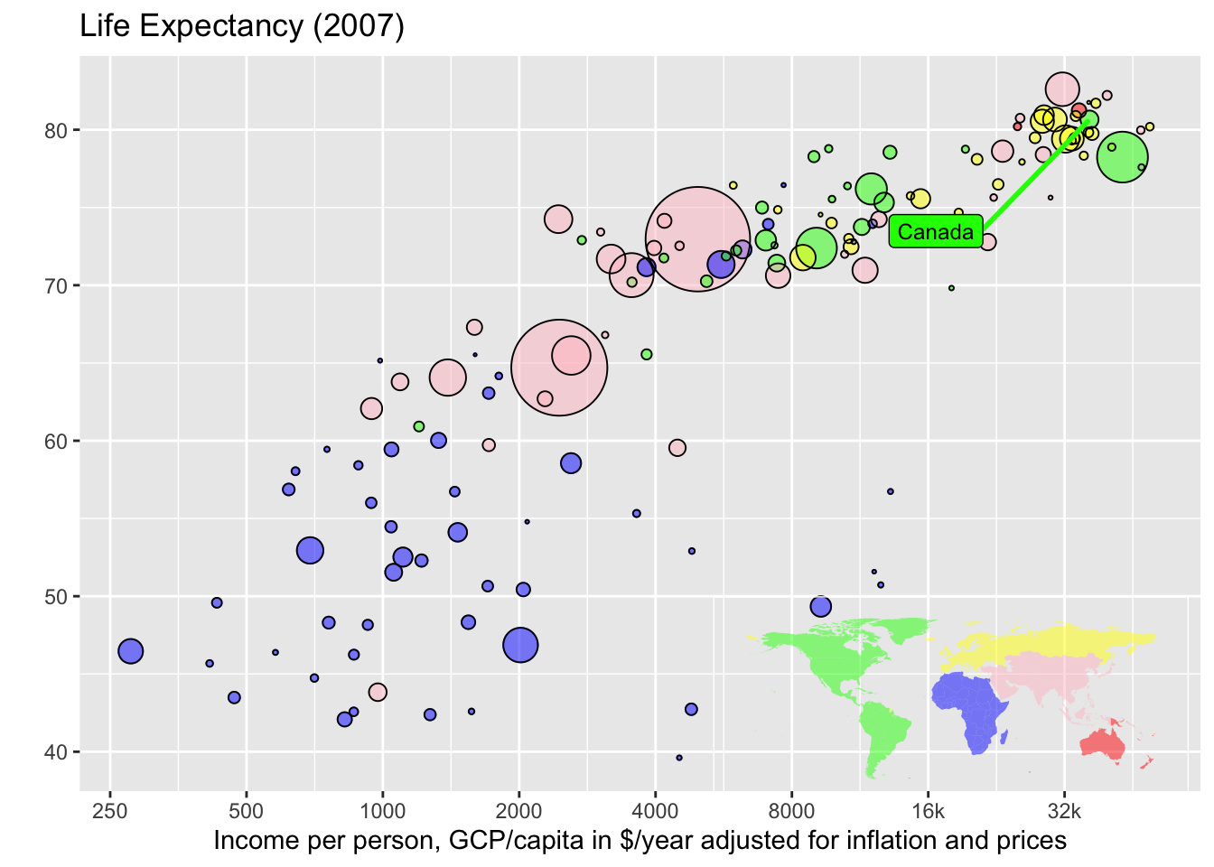
In addition to tidyverse and gapminder, in this lesson we used
ggrepelrnaturalearthrnaturalearthdataReconstruct the WeatherSpark visualization for a location in Canada using Environment Canada weather data.