32.1 Example plots for customization

We’ll use a couple of plots repeatedly: one with facets, and one with many other elements, but no facets.

p1 <- penguins %>% ggplot(aes(x = body_mass_g, y = flipper_length_mm, 
                              color = species, shape = sex)) + 
  geom_point()
p1

## Warning: Removed 11 rows containing missing values (geom_point).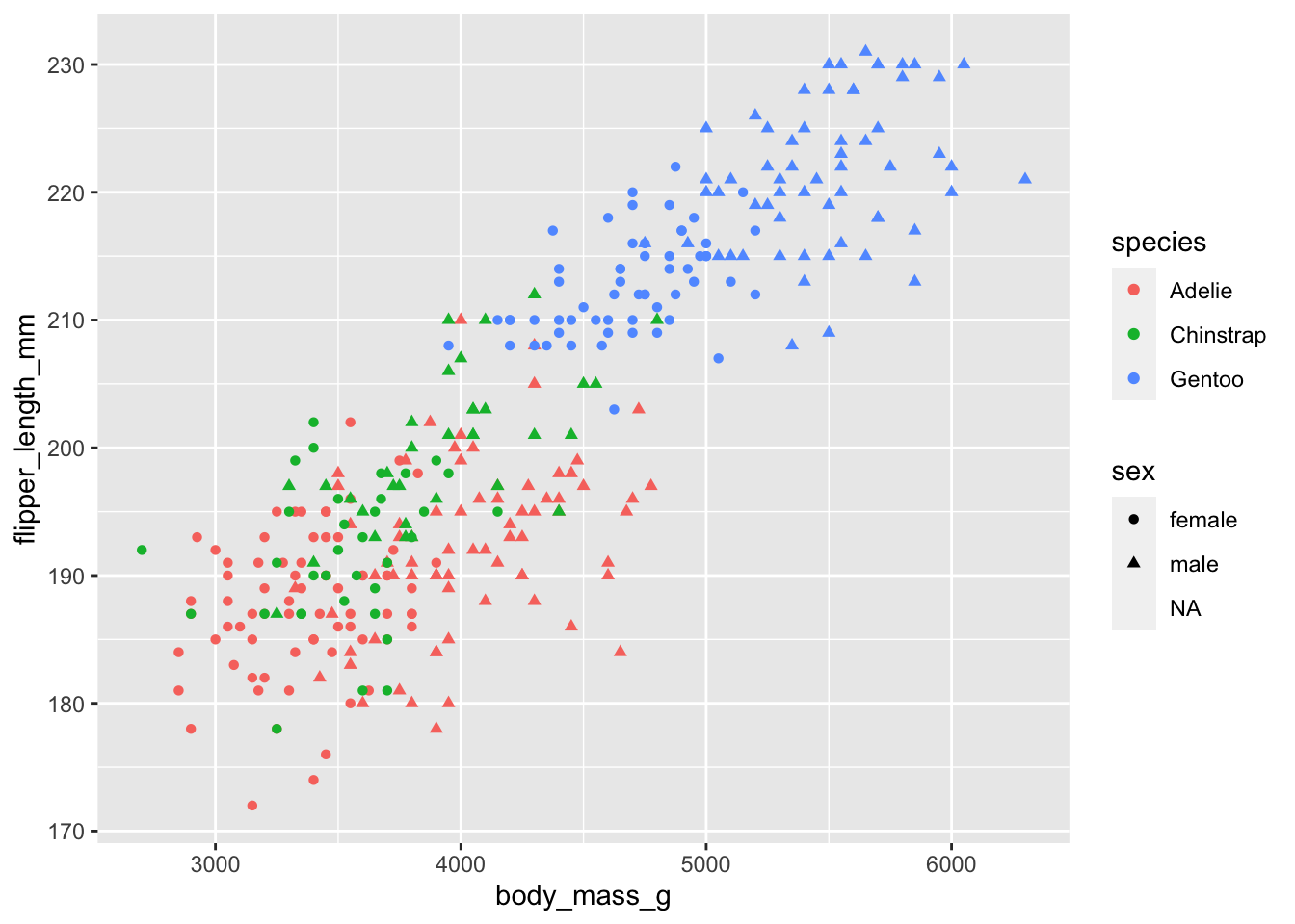

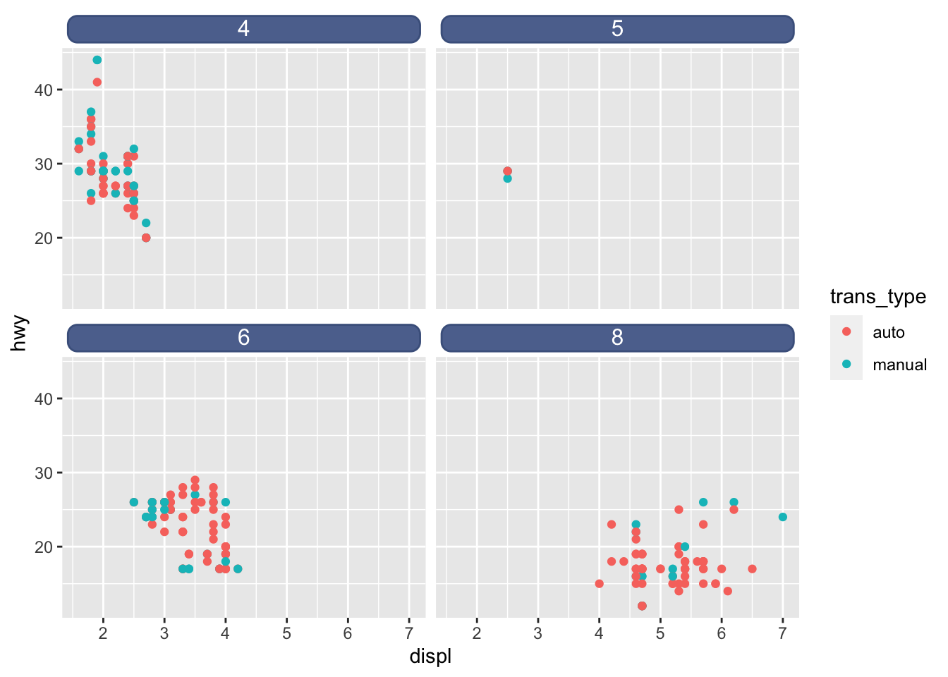
p2 <- mpg %>% 
  unglue_unnest(trans, "{trans_type}({trans_code})") %>%
           ggplot(aes(x = displ, y = hwy, color = trans_type)) +
                    geom_point() +
                    facet_wrap(~ factor(cyl))
p2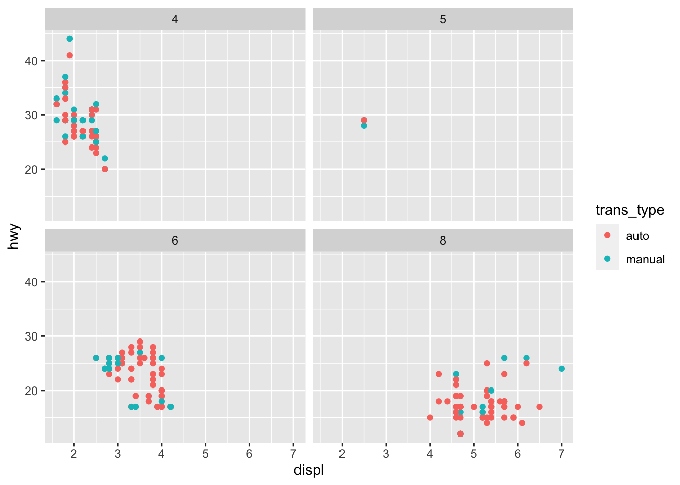

32.2 Built-in themes

There are many themes available that change the whole look of your plot. I’ve used theme_bw many times already, so here are a couple of other examples. For each you can use the base_size option (default value 11) to scale text elements and base_line_size to scale line elements of the figure.

p1 + theme_linedraw(base_size = 15, base_line_size = 0.2)

## Warning: Removed 11 rows containing missing values (geom_point).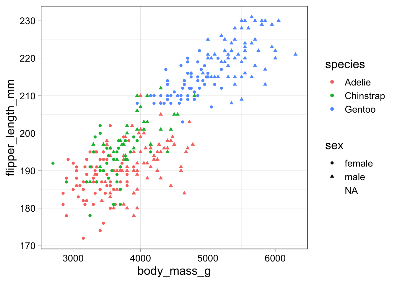

p2 + theme_dark(base_size = 20)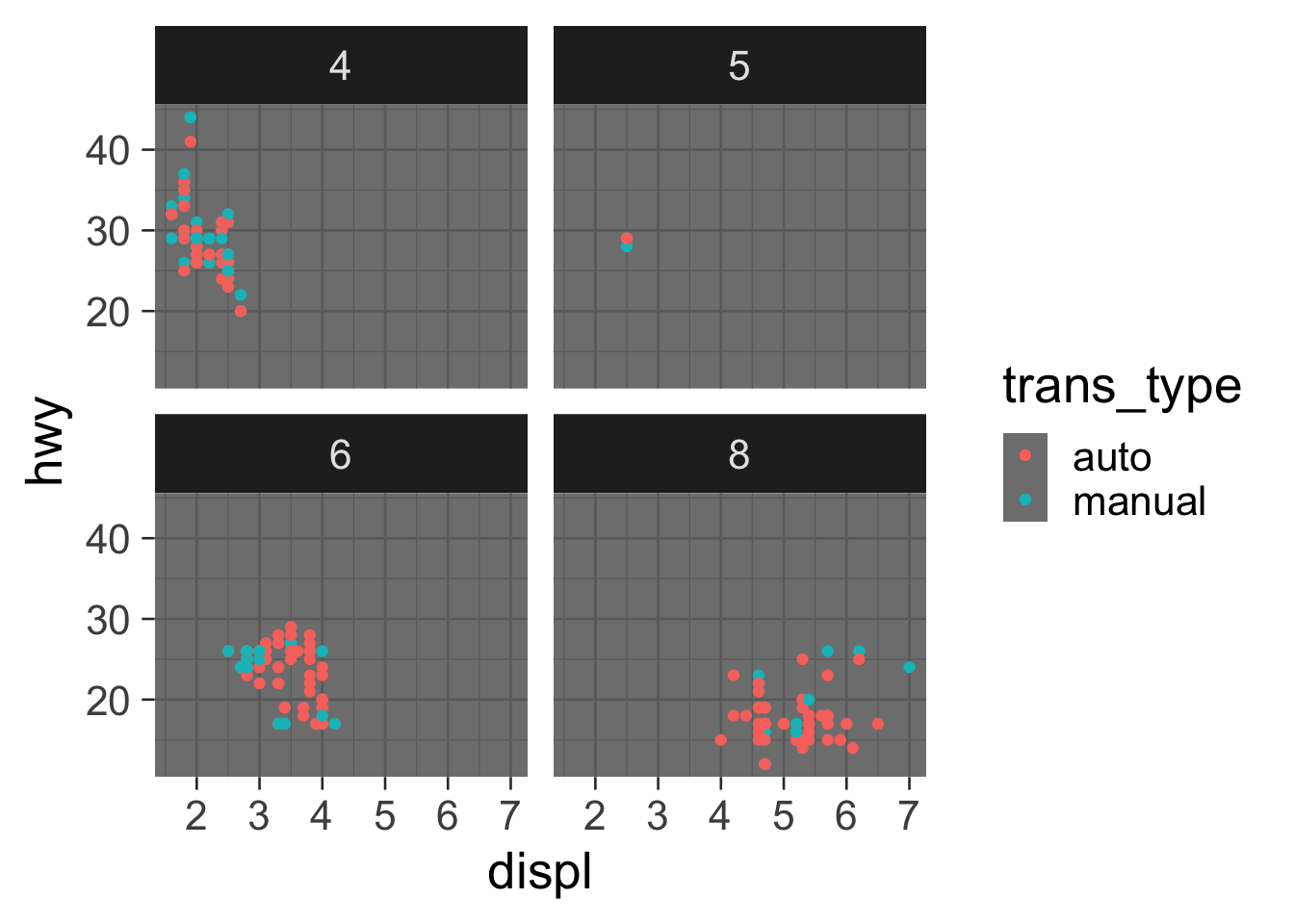

There are also add-in packages with more themes: ggthemes has theme_tufte and theme_economist

p1 + theme_economist() + scale_fill_economist()

## Warning: Removed 11 rows containing missing values (geom_point).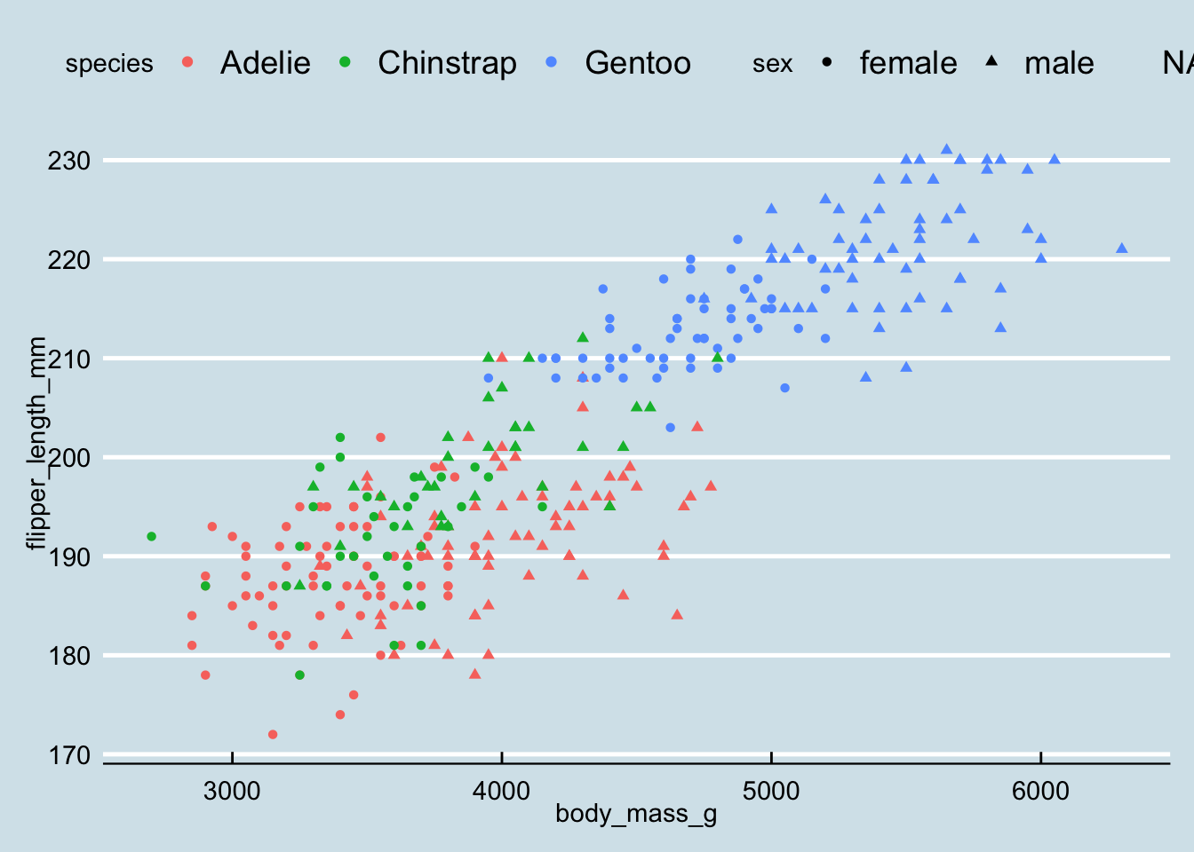

Another collection of themes is available in ggthemer. The main goal of this lesson is to give you the vocabulary and skills to customize the theme of your plot, so I won’t spend any more time on theme packages. On to the details!

32.3 Customizing text on a figure

The most common change I want to make to a plot’s theme (after axis and guide labels) is to increase the size of the text. This can be done using theme(text= ...) or for specific elements, theme(axis.title=...) (see the help page for more elements of the theme that can be set with a text element.) On the right side of the equals sign, you need the function element_text which allows you to control 10 different characteristics of your text. Here is an example of a few of the features.

Themes are controlled hierarchically, so adjusting text affects all text on the plot. Adjusting axis.title affects both axis.title.x and axis.title.y.

p2  + theme(text = element_text(size = 15),
            axis.text.x = element_text(angle = 45),
            axis.title.y = element_text(color = "blue"),
            strip.text = element_text(face = "bold"),
            legend.text = element_text(hjust = 1),
            legend.title = element_text(family = "serif"),
            axis.title.x = element_text(color = "#FF00FF", size = 18, face = "italic", family = "mono"))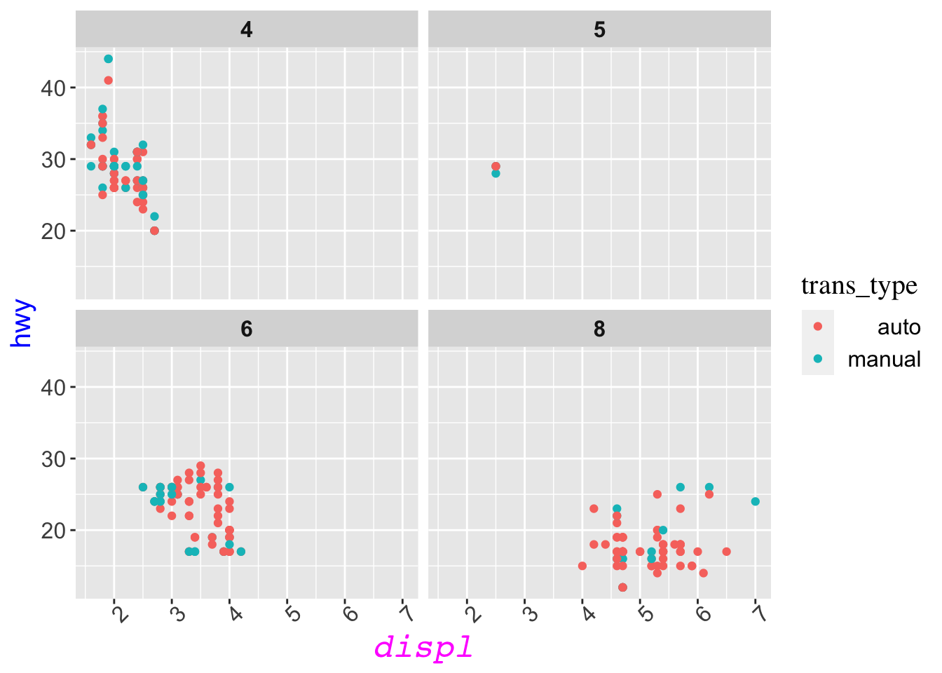

Compare this with the original version of the plot and play “spot the differences”.

32.4 Customizing borders, ticks, axis labels

There are many elements on a plot drawn with lines. These too can be customized all at once using theme(line = ...) or element by element using, for example theme(axis.line.x=...) or theme(axis.ticks.y=...). The grid lines can be adjusted using panel.grid.major and panel.grid.minor. These elements are named and controlled hierarchically as well. The right hand size of the expressions above must have an element_line function which allows you to control color, size, linetype and other features like arrows.

p2 + theme(line = element_line(size = 1),
           axis.ticks.y = element_line(color = "pink"),
           axis.line.x = element_line(linetype = 3, size = 0.25),
           panel.grid.minor.y = element_blank(),
           panel.grid.major = element_line(linetype = 3, color = "black", size = 0.25))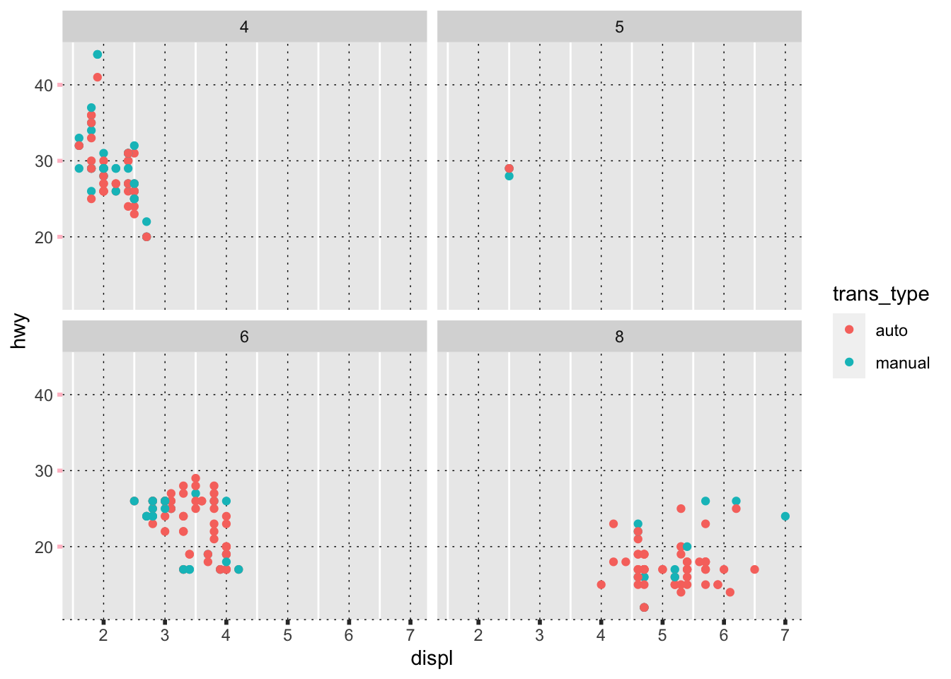

32.5 Enhanced text

The ggtext package allows you to use markdown and HTML code in any text element on your plot. You need to use element_markdown (or element_textbox_simple) instead of element_text for each element you want to use this enhanced formatting method with.

Unlike other theme elements, you can’t easily use ggtext formatting hierarchically: you can’t simply set all text to use elemment_markdown or even both axis labels. You must control each element individually.

p1 + labs(title = "_Penguin data from **Palmer station**, Antarctica_<sup>1</sup>",
          x = "<span style = 'color:red;'>body mass (g)</span>",
          y = "flipper length (mm)",
          caption = "<sup>1</sup>Collected by K. Gorman"
          ) + 
  theme(plot.title = element_markdown(lineheight = 1.2),
        plot.caption = element_markdown(),
        axis.title.x = element_textbox_simple(halign = 0.5)
        )

## Warning: Removed 11 rows containing missing values (geom_point).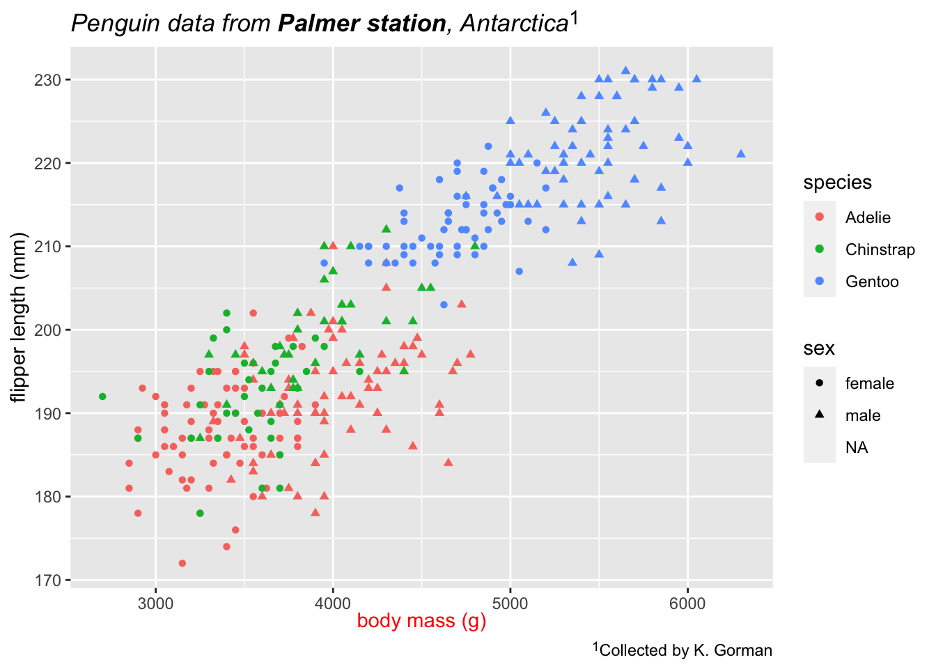

You can also add formatted boxes for the titles of facets and at any location on a plot.

p2 + theme(
    strip.background = element_blank(),
    strip.text = element_textbox(
      size = 12,
      color = "white", fill = "#5D729D", box.color = "#4A618C",
      halign = 0.5, linetype = 1, r = unit(5, "pt"), width = unit(1, "npc"),
      padding = margin(2, 0, 1, 0), margin = margin(3, 3, 3, 3)
    )
)

text_annotations <- tibble(
  label = c(
    "Some text **in bold.**",
    "Linebreaks<br>Linebreaks<br>Linebreaks",
    "*x*<sup>2</sup> + 5*x* + *C*<sub>*i*</sub>",
    "Some <span style='color:blue'>blue text **in bold.**</span>"
  ),
  x = c(4000, 5200, 5700, 5000),
  y = c(220, 200, 175, 150),
  hjust = c(0.5, 0, 0, 1),
  vjust = c(0.5, 1, 0, 0.5),
  angle = c(0, 0, 45, -45),
  # sex = c("male", "male", "male", "male")
)
p1 + geom_richtext(mapping = aes(x = x, y = y, label = label,
                                 angle = angle, hjust = hjust, vjust = vjust),
                   data = text_annotations,
                   inherit.aes = FALSE,
                   fill = NA,
                   color = "black")

## Warning: Removed 11 rows containing missing values (geom_point).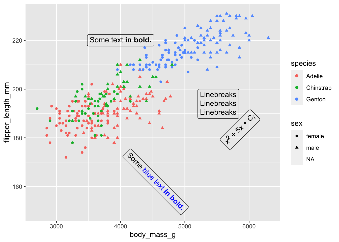

32.6 Further reading

• ggplot tidyverse documentation - like the theme help page, but shows the results of the examples
• Documentation for ggtext