28.1 Tiled maps with leaflet

In the previous lesson we made maps to show geographical data using map outlines from R packages. In this lesson we will look at making maps that build on detailed basemaps from online mapping systems. Google maps is a well known service; OpenStreetMap is a community-built free alternative. We will use the leaflet package.

Let’s make a map and place a marker at the location of the Mathematics and Statistics Department. You can pan and zoom this map from within Rstudio and in the knitted output.

m <- leaflet() %>%
  addTiles() %>%  # Add default OpenStreetMap map tiles
  addMarkers(lng=-63.5932, lat=44.63697, popup="Math & Stats, Dalhousie U")
m  # Print the map

Let’s use the city database we used in the MDS lesson to label the 61 cities we selected in that lesson.

cities <- read_csv("static/selected_cities.csv")

## 
## ── Column specification ────────────────────────────────────────────────────────
## cols(
##   city = col_character(),
##   city_ascii = col_character(),
##   lat = col_double(),
##   lng = col_double(),
##   country = col_character(),
##   iso2 = col_character(),
##   iso3 = col_character(),
##   admin_name = col_character(),
##   capital = col_character(),
##   population = col_double(),
##   id = col_double()
## )

m2 <- leaflet(data = cities) %>%
  addTiles() %>%
  addCircleMarkers(~ lng, ~lat, label = ~city)
m2

There are several different basemaps, or tiles, that you can use. A fun one to look at – because it changes frequently is a radar map for the USA from Iowa State.

m3 <- leaflet(data = cities) %>%
  addTiles() %>%
  addCircleMarkers(~ lng, ~lat, label = ~city) %>%
  addWMSTiles("http://mesonet.agron.iastate.edu/cgi-bin/wms/nexrad/n0r.cgi",
    layers = "nexrad-n0r-900913",
    options = WMSTileOptions(format = "image/png", transparent = TRUE),
    attribution = "Weather data © 2012 IEM Nexrad") %>%
  setView(-93.65, 42.0285, zoom = 4)
m3

It’s common to see “chloropleth” maps of the USA in which geographic regions are coloured to show a quantitative or categorical variable, such as population density or election results. These maps are less common in Canada due to two main factors: the geographic concentration of the population in cities means that area maps are even less informative than for the USA and the latitude range of Canada makes for some severe challenges when plotting whole-country territory and province chloropleth maps on commonly used projections. Nevertheless, it is possible. Here’s a demonstration with some random numbers for “data”.

library(geojsonio)

## Registered S3 method overwritten by 'geojsonsf':
##   method        from   
##   print.geojson geojson

## 
## Attaching package: 'geojsonio'

## The following object is masked from 'package:base':
## 
##     pretty

pal <- colorNumeric("viridis", NULL)  # make a viridis palette
canada <- geojson_read("https://gist.githubusercontent.com/mikelotis/2156d7c170d10d2c77cb79424fe2137d/raw/7a13748ed7ea5ba64876c77c53b6cb64dd5c3ab0/canada-province.geojson", what="sp")
my_values = runif(13, 0, 10) # random numbers between 0 and 10
canada %>% 
  leaflet() %>%
  addTiles() %>%
  addPolygons(fillColor = ~ pal(my_values)) %>%
  addLegend(pal = pal, values = my_values, opacity = 1.0)

28.2 Tiled map with ggmap

In this section we will use tile maps from the openstreetmap database rendered by Stamen Maps. We will use the ggmap package to download and draw the map.

There are two steps. First download the tiles needed for your map by specifying

• the bounding box in degrees latitude and longitude,
• the zoom level of the map, and
• the type of the tiles (terrain, terrain-background, etc. See the help for get_stamenmap for more.)

Always start with a small zoom level – if you make it too big you will download a lot of unnecessary data, which takes time and imposes a burden on the service.

mymap_terrain <- get_stamenmap(bbox = c(left = -130, bottom = 41, right = -50, top = 60), zoom=4, maptype = "terrain")

## Source : http://tile.stamen.com/terrain/4/2/4.png

## Source : http://tile.stamen.com/terrain/4/3/4.png

## Source : http://tile.stamen.com/terrain/4/4/4.png

## Source : http://tile.stamen.com/terrain/4/5/4.png

## Source : http://tile.stamen.com/terrain/4/2/5.png

## Source : http://tile.stamen.com/terrain/4/3/5.png

## Source : http://tile.stamen.com/terrain/4/4/5.png

## Source : http://tile.stamen.com/terrain/4/5/5.png

ggmap(mymap_terrain)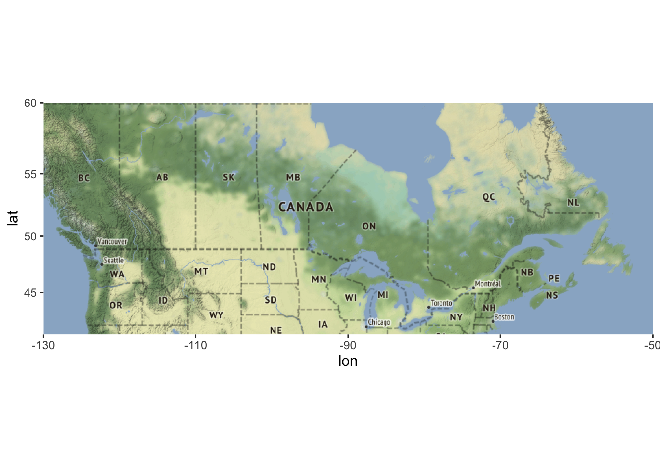  

This is a regular ggplot, so you can add lines and points to a map easily, using latitude and longitude as coordinates. Placing text on a map in a readable and attractive way can be quite a challenge.

my_points <- tibble(lat = c(43+57/60, 49+53/60),
                    lon = c(-59-55/60, -97-9/60),
                    label = c("Sable Is.", "Winnipeg")
)
ggmap(mymap_terrain)  +
  geom_point(data =my_points, color="brown") + 
  geom_text(data = my_points, aes(label=label))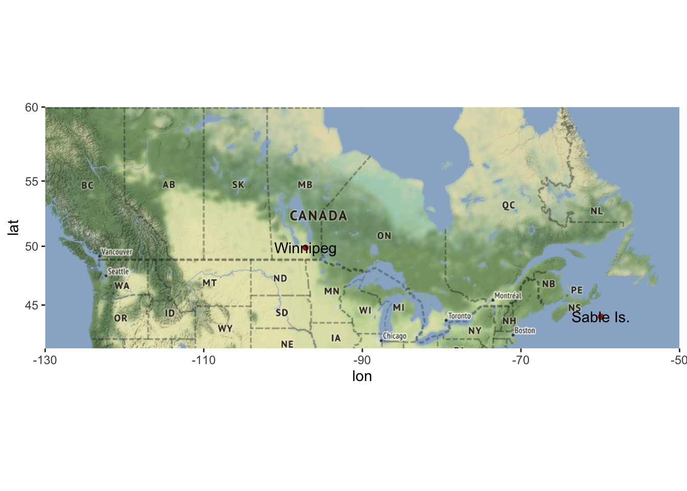

You can also zoom in on urban areas.

mymap_halifax <- get_stamenmap(bbox = c(left = -63.6-0.1, bottom = 44.60, right = -63.6+0.1, top = 44.75), 
                               zoom=12, maptype = "toner-lite")

## Source : http://tile.stamen.com/toner-lite/12/1323/1477.png

## Source : http://tile.stamen.com/toner-lite/12/1324/1477.png

## Source : http://tile.stamen.com/toner-lite/12/1325/1477.png

## Source : http://tile.stamen.com/toner-lite/12/1323/1478.png

## Source : http://tile.stamen.com/toner-lite/12/1324/1478.png

## Source : http://tile.stamen.com/toner-lite/12/1325/1478.png

## Source : http://tile.stamen.com/toner-lite/12/1323/1479.png

## Source : http://tile.stamen.com/toner-lite/12/1324/1479.png

## Source : http://tile.stamen.com/toner-lite/12/1325/1479.png

ggmap(mymap_halifax)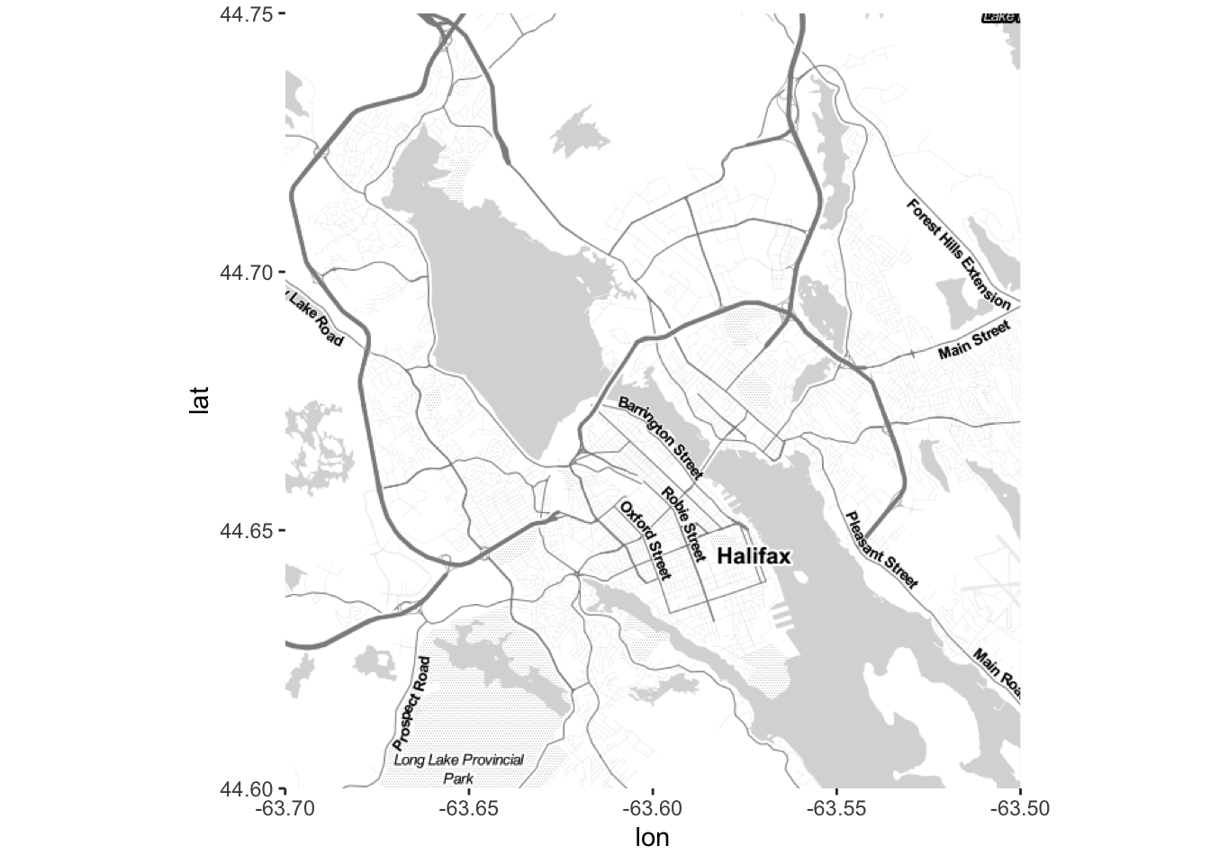  

28.3 Further reading

• Healy’s chapter 7 on mapping
• Wilke’s chapter 15 on geospatial data
• An article describing how ggmap works
• A ggmap tutorial, showing how to use Google map services including geocoding (turning an address into a location and the reverse) and routing.
• Another well-developed approach to mapping: mapview