Making sliding maps
2026-03-26
Plan
Kinds of maps (outline vs. tiles; interactive vs. static)
Creating basic maps
Adding points
Shading areas
Tile service providers
Map libraries
Dynamic:
leafletfor drawing raster or tiled maps (leafletjs.com)Static:
ggmap(part of tidyverse, tiles from several services)maptiles,tidyterra,sf-
Both rely on internet services such as:
A basic map
A basic map
Adding points
| city | city_ascii | lat | lng | country | iso2 | iso3 | admin_name | capital | population | id |
|---|---|---|---|---|---|---|---|---|---|---|
| Tokyo | Tokyo | 35.6897 | 139.6922 | Japan | JP | JPN | Tōkyō | primary | 37977000 | 1392685764 |
| Jakarta | Jakarta | -6.2146 | 106.8451 | Indonesia | ID | IDN | Jakarta | primary | 34540000 | 1360771077 |
| Delhi | Delhi | 28.6600 | 77.2300 | India | IN | IND | Delhi | admin | 29617000 | 1356872604 |
| Mumbai | Mumbai | 18.9667 | 72.8333 | India | IN | IND | Mahārāshtra | admin | 23355000 | 1356226629 |
Adding points
Colour regions with names
canada_map <- rnaturalearth::ne_states(country = "canada", returnclass = "sf")
pal <- colorFactor(palette = "viridis", domain = canada_map$name)
m3a <- leaflet(canada_map) |>
addTiles() |> # Standard OpenStreetMap background
addPolygons(
fillColor = ~pal(name), # Fill based on province name
fillOpacity = 0.7,
color = "white", # Border color
weight = 1, # Border thickness
highlightOptions = highlightOptions(
weight = 3, color = "#666",
bringToFront = TRUE),
label = ~name # Pop-up labels on hover
) |>
addLegend(
pal = pal, values = ~name,
title = "Province",
position = "bottomright" )Colour regions with names
Colour regions with numbers
pal <- colorNumeric("viridis", NULL) # make a viridis palette
my_values = runif(13, 0, 10) # random numbers between 0 and 10
m3b <- leaflet(canada_map) |>
addTiles() |> # Standard OpenStreetMap background
addPolygons(
fillColor = ~pal(my_values), # Fill based on province name
fillOpacity = 0.7,
color = "white", # Border color
weight = 1, # Border thickness
highlightOptions = highlightOptions(
weight = 3, color = "#666",
bringToFront = TRUE),
label = ~name # Pop-up labels on hover
) |>
addLegend(
pal = pal, values = ~my_values,
title = "Province",
position = "bottomright")Colour regions with numbers
Other tiled map services
Google maps have more options, but you must sign up for an API key first. These examples are for anyone who wants to experiment with that option.
See help for the package ggmap for more services (google maps, open street maps).
Start with a small integer for zoom and increase it if your map is fuzzy. (Don’t burden yourself or a free service by downloading unnecessary data.)
ESRI maps
library(maptiles)
library(tidyterra)
library(sf)
# 1. Define your area (Halifax to a broader view of Canada)
bbox_canada <- st_bbox(c(xmin = -130, ymin = 41, xmax = -50, ymax = 66), crs = 4326)
# 2. Get the tiles - "Esri.WorldTerrain" is high quality and key-free
# You can also try "OpenTopoMap" for more of a topographic contour look
terrain_tiles <- get_tiles(bbox_canada, provider = "Esri.WorldTerrain", zoom = 5)
m5a <- ggplot() +
geom_spatraster_rgb(data = terrain_tiles) +
theme_minimal() 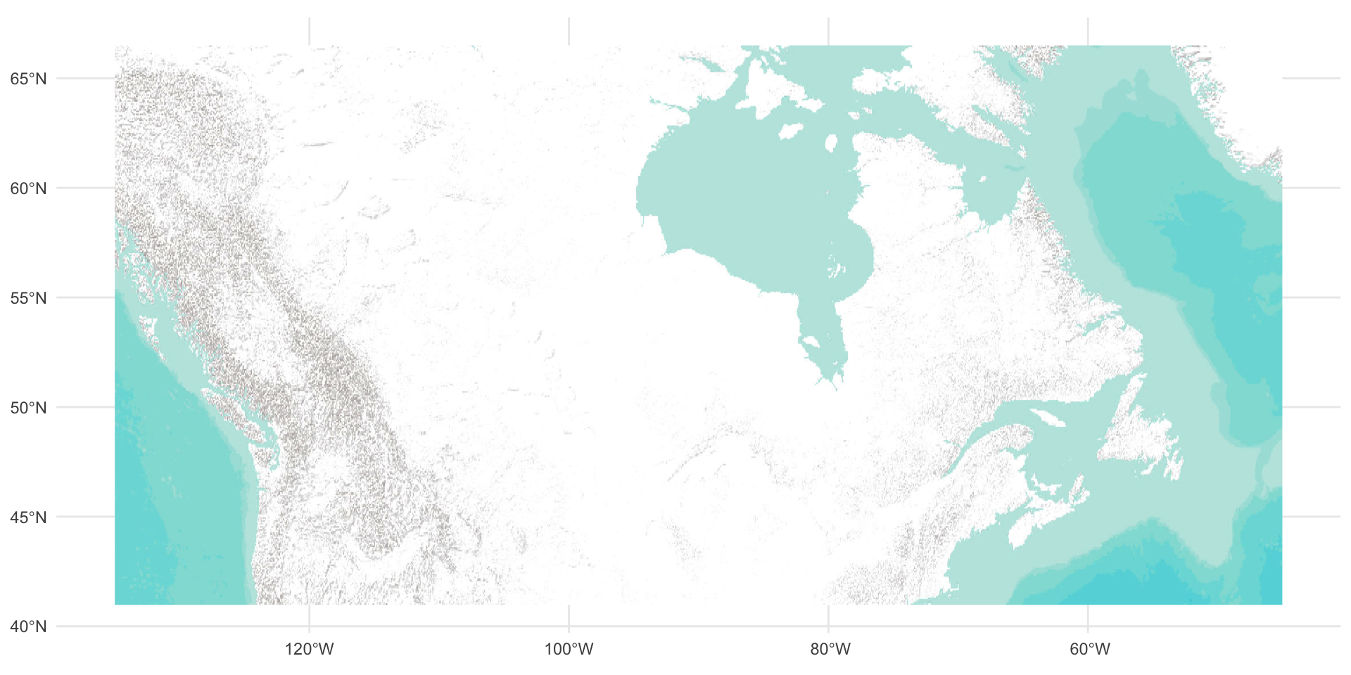
Add text and points
my_points <- tibble(lat = c(43+57/60, 49+53/60),
lon = c(-59-55/60, -97-9/60),
label = c("Sable Is.", "Winnipeg")
) |> st_as_sf(coords = c("lon", "lat"), crs = 4326)
m5 <- ggplot() +
geom_spatraster_rgb(data = terrain_tiles) +
geom_sf(data = my_points, color = "brown", size = 2) +
geom_sf_label(data = my_points,
aes(label = label),
fill = "#FFFFFF90",
color = "black") +
theme_minimal()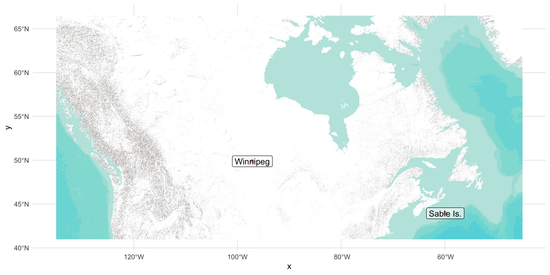
Summary
Outline vs tiled (image) maps
Make a basic map
Add points and labels
Fill regions with colour (requires polygons)
There are several tile services, but free access comes and goes frequently