Making outline maps

Andrew Irwin, a.irwin@dal.ca

2026-03-24

Plan

• Kinds of maps

• Basic maps

• Adding points

• Shading areas

• Projections

Map libraries

• sf for “simple (geographic) features`
• maps
• rnaturalearth and rnaturalearthdata (see naturalearthdata.com)
• cancensus for detailed maps of Canada
• mapproj for making projections of the Earth’s surface
• leaflet for drawing raster or tiled maps (next lesson)

Kinds of maps

• Coastlines and political boundaries

• Natural features (rivers, water bodies)

• Points and filled regions on maps

• Tiled maps

How to represent latitude and longitude from a sphere on a flat screen? (Projections.)

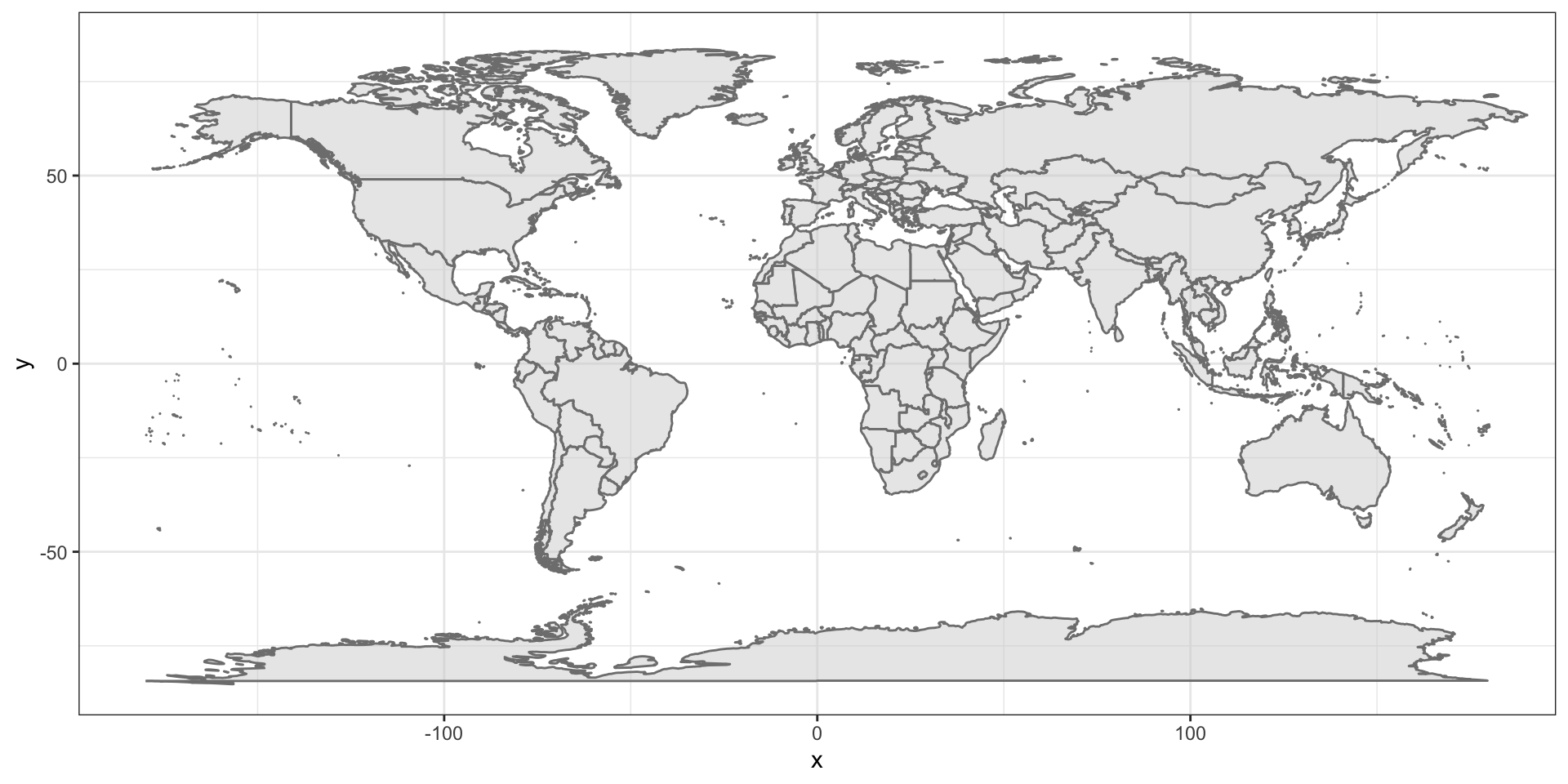
A basic map

library(tidyverse, quietly = TRUE)
library(sf)
library(maps)
WorldData <- maps::map(plot=FALSE, fill=TRUE)  |> st_as_sf()
m1 <- ggplot(WorldData) + 
  geom_sf(fill = "grey", color = "white", linewidth = 0.2) +
  theme_bw()

A basic map

Colour countries

WorldData <- WorldData |> mutate(value = runif(n()))
m2 <- WorldData |> ggplot() + 
        geom_sf(aes(fill = value),
                colour = "white", 
                linewidth=0.2) +
   theme_minimal()

Colour countries

Show only some countries

m3 <- WorldData |> 
  filter(ID %in% c("Canada", "China", "Chile")) |>
  ggplot() + 
    geom_sf(aes(fill = value),
             colour = "lightgray", 
             linewidth=0.2) +
  theme_void()

Show some countries

Colour some countries

values <- tibble( ID = c("Canada", "China", "Chile"),
                  value2  = c(1, 2, 3))
m4 <- WorldData |>
  left_join(values) |>
  ggplot() + 
       geom_sf(colour = "white", fill = "tan",
               linewidth=0.1) +
       geom_sf(aes(fill = value2), color = "white",
               linewidth = 0.1) + 
  scale_fill_continuous(na.value = "transparent") +
  theme_minimal()

Colour some countries

Add points

library(rnaturalearth)
library(rnaturalearthdata)
library(ggrepel)
canada <- ne_countries(country = "canada", scale = "large", 
                       returnclass = "sf")
sites <- tibble(longitude = c(-81, -80), 
                latitude = c(44, 45), 
                label = c("A", "B"))
m5 <- ggplot(data = canada) +
      geom_sf() +
      geom_point(data = sites, 
                 aes(x = longitude, y = latitude), 
                 size = 4, shape = 21, fill = "darkred") +
  geom_label_repel(data = sites, 
                   aes(x = longitude, y = latitude, 
                       label = label)) + 
  coord_sf(xlim = c(-140,-50), ylim = c(42,65))

Add points

Projections

m6 <- canada |> ggplot() + 
        geom_sf(fill = "lightgray", colour = "#7f7f7f") +
  theme_bw() +
  coord_sf(crs = st_crs(3978))  # Albers Conic Equal Area

Projections

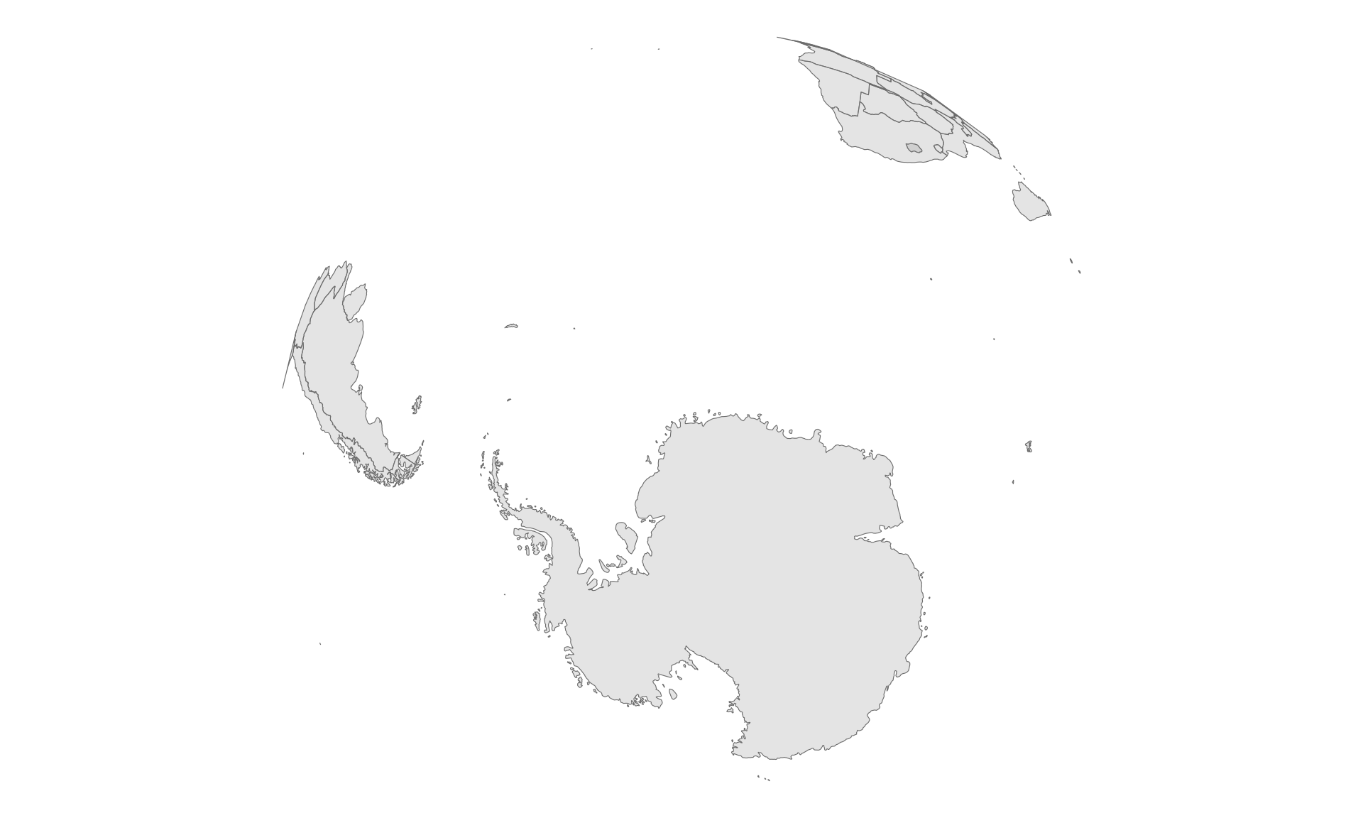
Polar regions

m7 <- WorldData |>
  ggplot() + 
        geom_sf(fill = "lightgray", colour = "#7f7f7f", 
                 alpha = 0.5, linewidth=0.2) +
  theme_bw() +
  coord_sf(crs = paste0("+proj=nsper +h=", 2.5 * 6371000, " +lat_0=60 +lon_0=-100"))

Polar regions

Other pole

m7a <- WorldData |>
  ggplot() + 
        geom_sf(fill = "lightgray", colour = "#7f7f7f", 
                 alpha = 0.5, linewidth=0.2) +
  theme_void() +
  coord_sf(crs = paste0("+proj=nsper +h=", 2.5 * 6371000, " +lat_0=-75 +lon_0=0"))

Polar regions

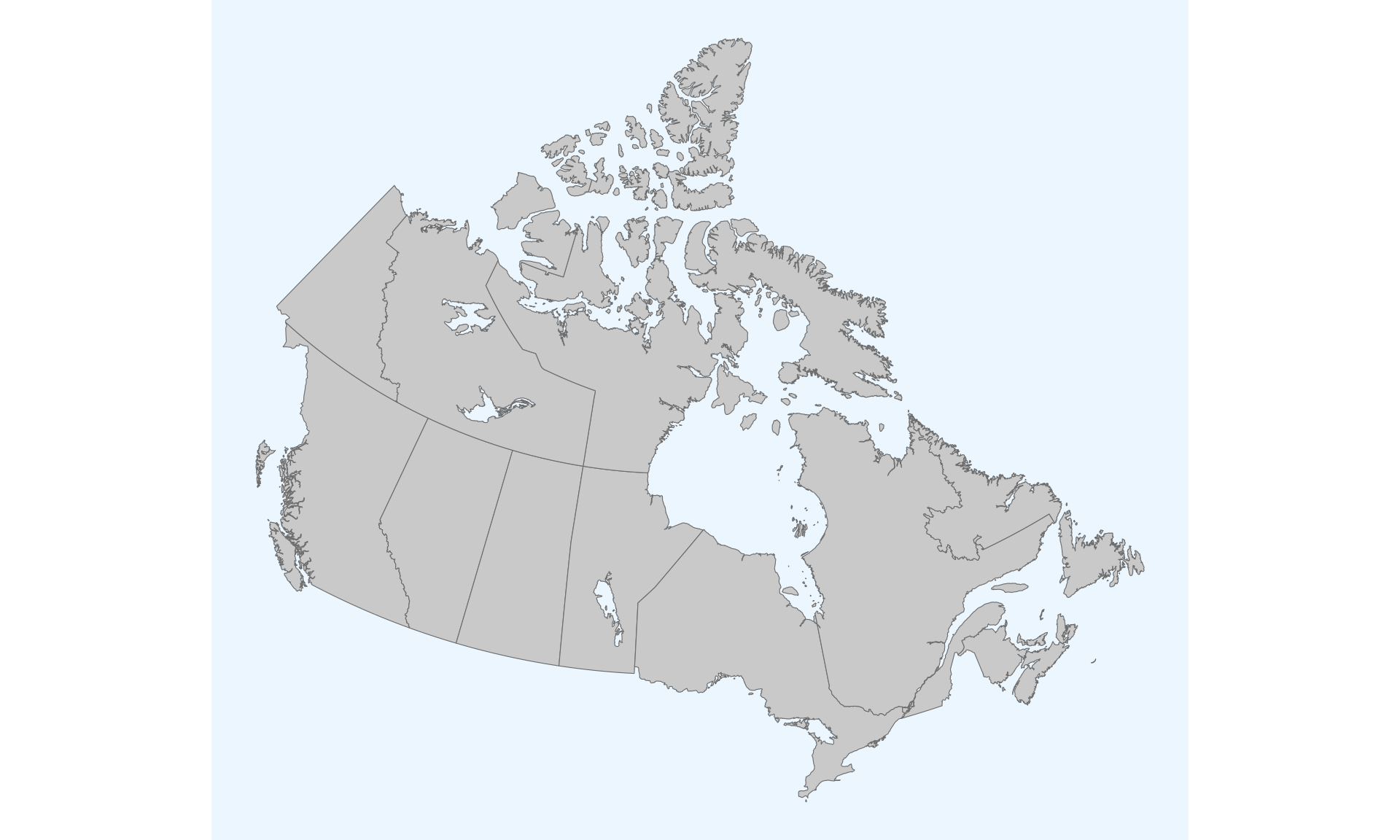
Map of Canada

With provinces and territories

canada <- ne_states(country = "canada", returnclass = "sf")
m8 <- canada |> ggplot() + 
        geom_sf(fill = "lightgray", colour = "#7f7f7f") +
    coord_sf(crs = st_crs(3347)) +  # Lambert Conformal
theme_void() +
  theme(
    panel.background = element_rect(fill = "aliceblue"),
    panel.grid = element_blank()
  )

Map of Canada with Census divisions

library(cancensus)
# set_cancensus_cache_path('/tmp', install = TRUE)
# https://censusmapper.ca/
# https://mountainmath.github.io/cancensus/index.html#api-key
canada_counties <- get_census(
  dataset = "CA21", 
  regions = list(C = "01"), 
  level = "CD", 
  geo_format = "sf"
)

Downloading: 16 kB     
Downloading: 16 kB     
Downloading: 33 kB     
Downloading: 33 kB     
Downloading: 33 kB     
Downloading: 33 kB     
Downloading: 66 kB     
Downloading: 66 kB     
Downloading: 66 kB     
Downloading: 66 kB     
Downloading: 82 kB     
Downloading: 82 kB     
Downloading: 82 kB     
Downloading: 82 kB     
Downloading: 82 kB     
Downloading: 82 kB     
Downloading: 130 kB     
Downloading: 130 kB     
Downloading: 150 kB     
Downloading: 150 kB     
Downloading: 160 kB     
Downloading: 160 kB     
Downloading: 180 kB     
Downloading: 180 kB     
Downloading: 200 kB     
Downloading: 200 kB     
Downloading: 200 kB     
Downloading: 200 kB     
Downloading: 200 kB     
Downloading: 200 kB     
Downloading: 200 kB     
Downloading: 200 kB     
Downloading: 210 kB     
Downloading: 210 kB     
Downloading: 210 kB     
Downloading: 210 kB     
Downloading: 230 kB     
Downloading: 230 kB     
Downloading: 230 kB     
Downloading: 230 kB     
Downloading: 240 kB     
Downloading: 240 kB     
Downloading: 240 kB     
Downloading: 240 kB     
Downloading: 240 kB     
Downloading: 240 kB     
Downloading: 260 kB     
Downloading: 260 kB     
Downloading: 260 kB     
Downloading: 260 kB     
Downloading: 260 kB     
Downloading: 260 kB     
Downloading: 260 kB     
Downloading: 260 kB     
Downloading: 280 kB     
Downloading: 280 kB     
Downloading: 280 kB     
Downloading: 280 kB     
Downloading: 280 kB     
Downloading: 280 kB     
Downloading: 280 kB     
Downloading: 280 kB     
Downloading: 290 kB     
Downloading: 290 kB     
Downloading: 290 kB     
Downloading: 290 kB     
Downloading: 290 kB     
Downloading: 290 kB     
Downloading: 290 kB     
Downloading: 290 kB     
Downloading: 310 kB     
Downloading: 310 kB     
Downloading: 310 kB     
Downloading: 310 kB     
Downloading: 310 kB     
Downloading: 310 kB     
Downloading: 310 kB     
Downloading: 310 kB     
Downloading: 310 kB     
Downloading: 310 kB     
Downloading: 330 kB     
Downloading: 330 kB     
Downloading: 330 kB     
Downloading: 330 kB     
Downloading: 330 kB     
Downloading: 330 kB     
Downloading: 330 kB     
Downloading: 330 kB     
Downloading: 330 kB     
Downloading: 330 kB     
Downloading: 330 kB     
Downloading: 330 kB     
Downloading: 340 kB     
Downloading: 340 kB     
Downloading: 340 kB     
Downloading: 340 kB     
Downloading: 340 kB     
Downloading: 340 kB     
Downloading: 340 kB     
Downloading: 340 kB     
Downloading: 340 kB     
Downloading: 340 kB     
Downloading: 340 kB     
Downloading: 340 kB     
Downloading: 360 kB     
Downloading: 360 kB     
Downloading: 360 kB     
Downloading: 360 kB     
Downloading: 360 kB     
Downloading: 360 kB     
Downloading: 360 kB     
Downloading: 360 kB     
Downloading: 360 kB     
Downloading: 360 kB     
Downloading: 360 kB     
Downloading: 360 kB     
Downloading: 380 kB     
Downloading: 380 kB     
Downloading: 380 kB     
Downloading: 380 kB     
Downloading: 380 kB     
Downloading: 380 kB     
Downloading: 380 kB     
Downloading: 380 kB     
Downloading: 380 kB     
Downloading: 380 kB     
Downloading: 380 kB     
Downloading: 380 kB     
Downloading: 380 kB     
Downloading: 380 kB     
Downloading: 390 kB     
Downloading: 390 kB     
Downloading: 390 kB     
Downloading: 390 kB     
Downloading: 390 kB     
Downloading: 390 kB     
Downloading: 390 kB     
Downloading: 390 kB     
Downloading: 390 kB     
Downloading: 390 kB     
Downloading: 390 kB     
Downloading: 390 kB     
Downloading: 410 kB     
Downloading: 410 kB     
Downloading: 440 kB     
Downloading: 440 kB     
Downloading: 490 kB     
Downloading: 490 kB     
Downloading: 540 kB     
Downloading: 540 kB     
Downloading: 550 kB     
Downloading: 550 kB     
Downloading: 590 kB     
Downloading: 590 kB     
Downloading: 640 kB     
Downloading: 640 kB     
Downloading: 710 kB     
Downloading: 710 kB     
Downloading: 760 kB     
Downloading: 760 kB     
Downloading: 800 kB     
Downloading: 800 kB     
Downloading: 830 kB     
Downloading: 830 kB     
Downloading: 870 kB     
Downloading: 870 kB     
Downloading: 870 kB     
Downloading: 870 kB     
Downloading: 910 kB     
Downloading: 910 kB     
Downloading: 960 kB     
Downloading: 960 kB     
Downloading: 1 MB     
Downloading: 1 MB     
Downloading: 1.1 MB     
Downloading: 1.1 MB     
Downloading: 1.1 MB     
Downloading: 1.1 MB     
Downloading: 1.2 MB     
Downloading: 1.2 MB     
Downloading: 1.2 MB     
Downloading: 1.2 MB     
Downloading: 1.2 MB     
Downloading: 1.2 MB     
Downloading: 1.2 MB     
Downloading: 1.2 MB     
Downloading: 1.3 MB     
Downloading: 1.3 MB     
Downloading: 1.3 MB     
Downloading: 1.3 MB     
Downloading: 1.4 MB     
Downloading: 1.4 MB     
Downloading: 1.4 MB     
Downloading: 1.4 MB     
Downloading: 1.5 MB     
Downloading: 1.5 MB     
Downloading: 1.5 MB     
Downloading: 1.5 MB     
Downloading: 1.6 MB     
Downloading: 1.6 MB     
Downloading: 1.6 MB     
Downloading: 1.6 MB     
Downloading: 1.6 MB     
Downloading: 1.6 MB     
Downloading: 1.7 MB     
Downloading: 1.7 MB     
Downloading: 1.7 MB     
Downloading: 1.7 MB     
Downloading: 1.7 MB     
Downloading: 1.7 MB     
Downloading: 1.7 MB     
Downloading: 1.7 MB     
Downloading: 1.8 MB     
Downloading: 1.8 MB     
Downloading: 1.8 MB     
Downloading: 1.8 MB     
Downloading: 1.9 MB     
Downloading: 1.9 MB     
Downloading: 2 MB     
Downloading: 2 MB     
Downloading: 2 MB     
Downloading: 2 MB     
Downloading: 2 MB     
Downloading: 2 MB     
Downloading: 2 MB     
Downloading: 2 MB     
Downloading: 2 MB     
Downloading: 2 MB     
Downloading: 2.1 MB     
Downloading: 2.1 MB     
Downloading: 2.1 MB     
Downloading: 2.1 MB     
Downloading: 2.1 MB     
Downloading: 2.1 MB     
Downloading: 2.1 MB     
Downloading: 2.1 MB     
Downloading: 2.2 MB     
Downloading: 2.2 MB     
Downloading: 2.2 MB     
Downloading: 2.2 MB     
Downloading: 2.3 MB     
Downloading: 2.3 MB     
Downloading: 2.3 MB     
Downloading: 2.3 MB     
Downloading: 2.4 MB     
Downloading: 2.4 MB     
Downloading: 2.5 MB     
Downloading: 2.5 MB     
Downloading: 2.5 MB     
Downloading: 2.5 MB     
Downloading: 2.6 MB     
Downloading: 2.6 MB     
Downloading: 2.6 MB     
Downloading: 2.6 MB     
Downloading: 2.6 MB     
Downloading: 2.6 MB     
Downloading: 2.7 MB     
Downloading: 2.7 MB     
Downloading: 2.7 MB     
Downloading: 2.7 MB     
Downloading: 2.7 MB     
Downloading: 2.7 MB     
Downloading: 2.7 MB     
Downloading: 2.7 MB     
Downloading: 2.8 MB     
Downloading: 2.8 MB     
Downloading: 2.8 MB     
Downloading: 2.8 MB     
Downloading: 2.8 MB     
Downloading: 2.8 MB     
Downloading: 2.8 MB     
Downloading: 2.8 MB     
Downloading: 2.9 MB     
Downloading: 2.9 MB     
Downloading: 2.9 MB     
Downloading: 2.9 MB     
Downloading: 2.9 MB     
Downloading: 2.9 MB     
Downloading: 2.9 MB     
Downloading: 2.9 MB     
Downloading: 3 MB     
Downloading: 3 MB     
Downloading: 3 MB     
Downloading: 3 MB     
Downloading: 3 MB     
Downloading: 3 MB     
Downloading: 3.1 MB     
Downloading: 3.1 MB     
Downloading: 3.1 MB     
Downloading: 3.1 MB     
Downloading: 3.1 MB     
Downloading: 3.1 MB     
Downloading: 3.1 MB     
Downloading: 3.1 MB     
Downloading: 3.2 MB     
Downloading: 3.2 MB     
Downloading: 3.2 MB     
Downloading: 3.2 MB     
Downloading: 3.2 MB     
Downloading: 3.2 MB     
Downloading: 3.3 MB     
Downloading: 3.3 MB     
Downloading: 3.3 MB     
Downloading: 3.3 MB     
Downloading: 3.4 MB     
Downloading: 3.4 MB     
Downloading: 3.4 MB     
Downloading: 3.4 MB     
Downloading: 3.4 MB     
Downloading: 3.4 MB     
Downloading: 3.4 MB     
Downloading: 3.4 MB     
Downloading: 3.5 MB     
Downloading: 3.5 MB     
Downloading: 3.5 MB     
Downloading: 3.5 MB     
Downloading: 3.5 MB     
Downloading: 3.5 MB     
Downloading: 3.6 MB     
Downloading: 3.6 MB     
Downloading: 3.6 MB     
Downloading: 3.6 MB     
Downloading: 3.6 MB     
Downloading: 3.6 MB     
Downloading: 3.6 MB     
Downloading: 3.6 MB     
Downloading: 3.6 MB     
Downloading: 3.6 MB     
Downloading: 3.6 MB     
Downloading: 3.6 MB     
Downloading: 3.7 MB     
Downloading: 3.7 MB     
Downloading: 3.7 MB     
Downloading: 3.7 MB     
Downloading: 3.8 MB     
Downloading: 3.8 MB     
Downloading: 3.8 MB     
Downloading: 3.8 MB     
Downloading: 3.9 MB     
Downloading: 3.9 MB     
Downloading: 3.9 MB     
Downloading: 3.9 MB     
Downloading: 3.9 MB     
Downloading: 3.9 MB     
Downloading: 4 MB     
Downloading: 4 MB     
Downloading: 4 MB     
Downloading: 4 MB     
Downloading: 4 MB     
Downloading: 4 MB     
Downloading: 4 MB     
Downloading: 4 MB     
Downloading: 4.1 MB     
Downloading: 4.1 MB     
Downloading: 4.1 MB     
Downloading: 4.1 MB     
Downloading: 4.1 MB     
Downloading: 4.1 MB     
Downloading: 4.1 MB     
Downloading: 4.1 MB     
Downloading: 4.2 MB     
Downloading: 4.2 MB     
Downloading: 4.2 MB     
Downloading: 4.2 MB     
Downloading: 4.2 MB     
Downloading: 4.2 MB     
Downloading: 4.2 MB     
Downloading: 4.2 MB     
Downloading: 4.3 MB     
Downloading: 4.3 MB     
Downloading: 4.3 MB     
Downloading: 4.3 MB     
Downloading: 4.3 MB     
Downloading: 4.3 MB     
Downloading: 4.4 MB     
Downloading: 4.4 MB     
Downloading: 4.4 MB     
Downloading: 4.4 MB     
Downloading: 4.5 MB     
Downloading: 4.5 MB     
Downloading: 4.5 MB     
Downloading: 4.5 MB     
Downloading: 4.5 MB     
Downloading: 4.5 MB     
Downloading: 4.6 MB     
Downloading: 4.6 MB     
Downloading: 4.6 MB     
Downloading: 4.6 MB     
Downloading: 4.6 MB     
Downloading: 4.6 MB     
Downloading: 4.6 MB     
Downloading: 4.6 MB     
Downloading: 4.7 MB     
Downloading: 4.7 MB     
Downloading: 4.7 MB     
Downloading: 4.7 MB     
Downloading: 4.7 MB     
Downloading: 4.7 MB     
Downloading: 4.7 MB     
Downloading: 4.7 MB     
Downloading: 4.7 MB     
Downloading: 4.7 MB     
Downloading: 4.8 MB     
Downloading: 4.8 MB     
Downloading: 4.8 MB     
Downloading: 4.8 MB     
Downloading: 4.8 MB     
Downloading: 4.8 MB     
Downloading: 4.8 MB     
Downloading: 4.8 MB     
Downloading: 4.9 MB     
Downloading: 4.9 MB     
Downloading: 4.9 MB     
Downloading: 4.9 MB     
Downloading: 4.9 MB     
Downloading: 4.9 MB     
Downloading: 5 MB     
Downloading: 5 MB     
Downloading: 5 MB     
Downloading: 5 MB     
Downloading: 5 MB     
Downloading: 5 MB     
Downloading: 5 MB     
Downloading: 5 MB     
Downloading: 5.1 MB     
Downloading: 5.1 MB     
Downloading: 5.2 MB     
Downloading: 5.2 MB     
Downloading: 5.2 MB     
Downloading: 5.2 MB     
Downloading: 5.2 MB     
Downloading: 5.2 MB     
Downloading: 5.2 MB     
Downloading: 5.2 MB     
Downloading: 5.2 MB     
Downloading: 5.2 MB     
Downloading: 5.3 MB     
Downloading: 5.3 MB     
Downloading: 5.3 MB     
Downloading: 5.3 MB     
Downloading: 5.3 MB     
Downloading: 5.3 MB     
Downloading: 5.4 MB     
Downloading: 5.4 MB     
Downloading: 5.4 MB     
Downloading: 5.4 MB     
Downloading: 5.4 MB     
Downloading: 5.4 MB     
Downloading: 5.4 MB     
Downloading: 5.4 MB     
Downloading: 5.5 MB     
Downloading: 5.5 MB     
Downloading: 5.5 MB     
Downloading: 5.5 MB     
Downloading: 5.5 MB     
Downloading: 5.5 MB     
Downloading: 5.5 MB     
Downloading: 5.5 MB     
Downloading: 5.6 MB     
Downloading: 5.6 MB     
Downloading: 5.6 MB     
Downloading: 5.6 MB     
Downloading: 5.7 MB     
Downloading: 5.7 MB     
Downloading: 5.7 MB     
Downloading: 5.7 MB     
Downloading: 5.7 MB     
Downloading: 5.7 MB     
Downloading: 5.8 MB     
Downloading: 5.8 MB     
Downloading: 5.8 MB     
Downloading: 5.8 MB     
Downloading: 5.8 MB     
Downloading: 5.8 MB     
Downloading: 5.8 MB     
Downloading: 5.8 MB     
Downloading: 5.9 MB     
Downloading: 5.9 MB     
Downloading: 5.9 MB     
Downloading: 5.9 MB     
Downloading: 5.9 MB     
Downloading: 5.9 MB     
Downloading: 5.9 MB     
Downloading: 5.9 MB     
Downloading: 6 MB     
Downloading: 6 MB     
Downloading: 6 MB     
Downloading: 6 MB     
Downloading: 6 MB     
Downloading: 6 MB     
Downloading: 6 MB     
Downloading: 6 MB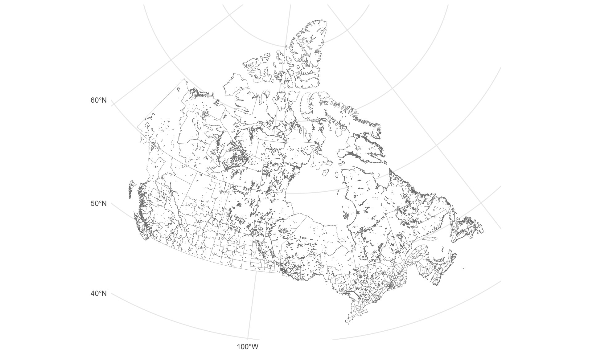     

m9 <- ggplot(data = canada_counties) +
  geom_sf(fill = "white", color = "gray50", size = 0.1) +
  coord_sf(crs = 3347) + 
  theme_minimal()

Population density

# v_CA21_6 is the vector for Population Density in the 2021 Census
# You can find vector IDs using: list_census_vectors("CA21")
pop_data <- get_census(
  dataset = "CA21", level = "CD",
  regions = list(C = "01"),
  vectors = c("pop_density" = "v_CA21_6"),
  geo_format = "sf")

Downloading: 8.4 kB     
Downloading: 8.4 kB     
Downloading: 8.4 kB     
Downloading: 8.4 kB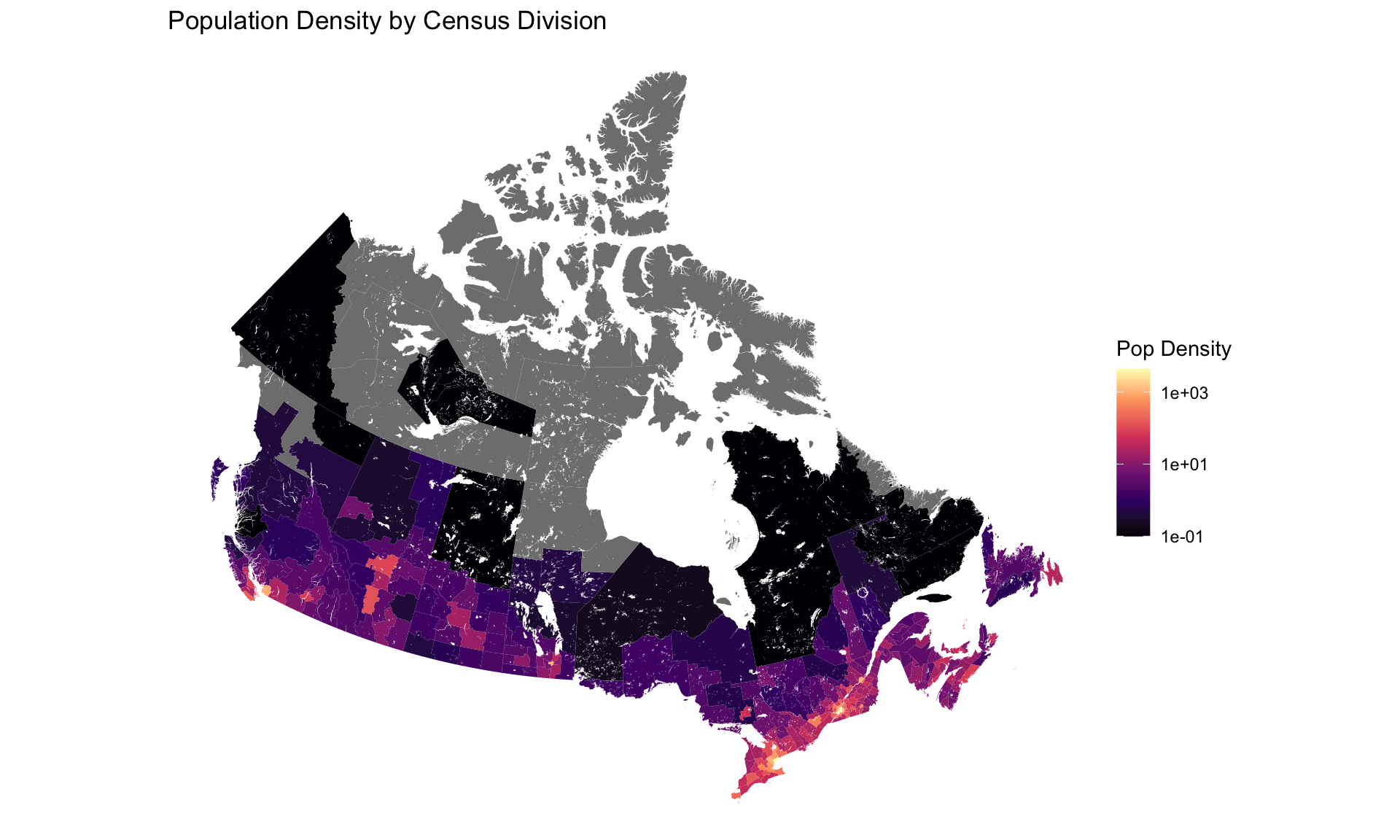     

m10 <- ggplot(pop_data) +
  geom_sf(aes(fill = pop_density), color = NA) +
  scale_fill_viridis_c(
    name = "Pop Density", 
    trans = "log10", option = "magma") +
  coord_sf(crs = 3347) +
  theme_void() +
  labs(title = "Population Density by Census Division")

Summary

• Make a basic map

• Select all or some countries

• Fill regions with colour

• Add points and labels

• Use a different projection

Exercises

• Make some simple maps following the examples in these slides and the course notes