2024-03-06
What is PCA and why do we use it?
Demonstration with gapminder data in 3 dimensions
More demonstrations
A tool for simplifying data sets with many variables down to a small number
Works best with quantitative variables that are partially correlated
Can be used with one or more categorical variables to identify subgroups
Main results are
Be careful with scaling and units
Plot made with plot_ly
function in plotly
package.
ggpairs
is in the GGally
package.
This matrix tells you how to rotate the data into PC coordinates which is the weight of each original variable in the computation of PCs.
pca2 %>% tidy(matrix="loadings") |> # same as rotation
filter(PC < 3) |>
pivot_wider(values_from="value",
names_from="PC", names_prefix="PC_") |> kable() |> kable_styling(full_width = FALSE)
column | PC_1 | PC_2 |
---|---|---|
Culmen Length (mm) | 0.2871721 | 0.6602934 |
Culmen Depth (mm) | -0.4102740 | 0.1879624 |
Flipper Length (mm) | 0.5008652 | 0.2207240 |
Body Mass (g) | 0.4846484 | 0.2033560 |
Delta 15 N (o/oo) | -0.4084370 | 0.3686830 |
Delta 13 C (o/oo) | -0.3108644 | 0.5501663 |
Use PCA to reduce the number of dimensions (variables) in your data
Interpret loadings (arrows and numeric vectors)
Pay attention to the proportion of variance along each principal component
Consequences of scaling variables (or not scaling them)
See the course notes for more code examples.
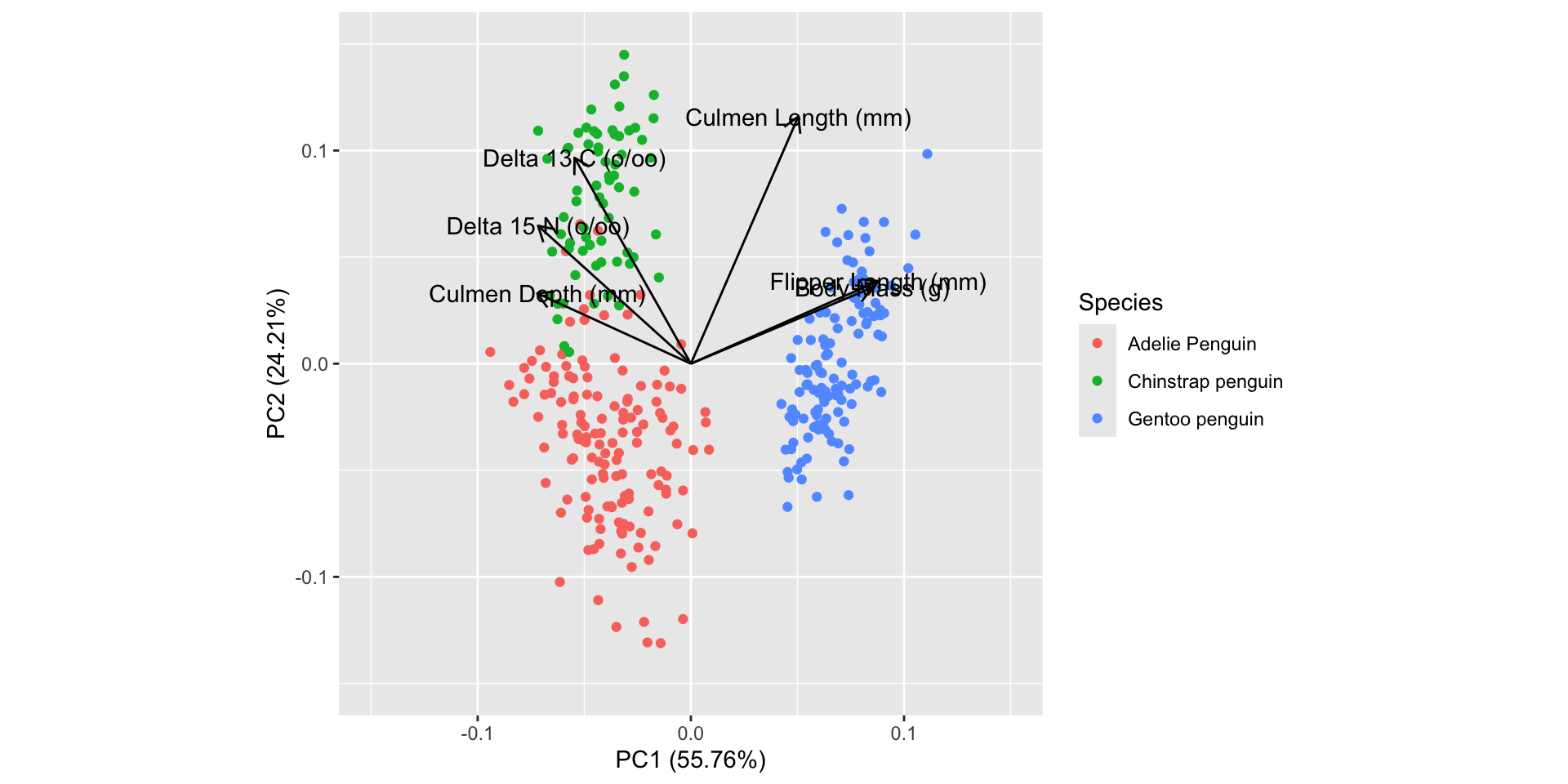
my_penguins_raw = penguins_raw |> select(-`Sample Number`) |>
select(Species, where(is.numeric) ) |> na.omit() |>
mutate(Species = str_remove(Species, "\\(.*\\)"))
pca2 <- my_penguins_raw |> select(-Species) |> prcomp(scale=TRUE)
autoplot(pca2, data = my_penguins_raw,
loadings=TRUE, loadings.label = TRUE,
loadings.label.colour = "black", loadings.colour = "black",
colour = 'Species') + xlim(-0.15, 0.15) + ylim(-0.15, 0.15)