Making your first plot

Andrew Irwin, a.irwin@dal.ca

2026-01-15

Use the ggplot2 library

Do this once (if you haven’t done it already):

install.packages("tidyverse")

Add this line to every Quarto document:

library(tidyverse)

Get some data

glimpse(mtcars)

Rows: 32
Columns: 11
$ mpg  <dbl> 21.0, 21.0, 22.8, 21.4, 18.7, 18.1, 14.3, 24.4, 22.8, 19.2, 17.8,…
$ cyl  <dbl> 6, 6, 4, 6, 8, 6, 8, 4, 4, 6, 6, 8, 8, 8, 8, 8, 8, 4, 4, 4, 4, 8,…
$ disp <dbl> 160.0, 160.0, 108.0, 258.0, 360.0, 225.0, 360.0, 146.7, 140.8, 16…
$ hp   <dbl> 110, 110, 93, 110, 175, 105, 245, 62, 95, 123, 123, 180, 180, 180…
$ drat <dbl> 3.90, 3.90, 3.85, 3.08, 3.15, 2.76, 3.21, 3.69, 3.92, 3.92, 3.92,…
$ wt   <dbl> 2.620, 2.875, 2.320, 3.215, 3.440, 3.460, 3.570, 3.190, 3.150, 3.…
$ qsec <dbl> 16.46, 17.02, 18.61, 19.44, 17.02, 20.22, 15.84, 20.00, 22.90, 18…
$ vs   <dbl> 0, 0, 1, 1, 0, 1, 0, 1, 1, 1, 1, 0, 0, 0, 0, 0, 0, 1, 1, 1, 1, 0,…
$ am   <dbl> 1, 1, 1, 0, 0, 0, 0, 0, 0, 0, 0, 0, 0, 0, 0, 0, 0, 1, 1, 1, 0, 0,…
$ gear <dbl> 4, 4, 4, 3, 3, 3, 3, 4, 4, 4, 4, 3, 3, 3, 3, 3, 3, 4, 4, 4, 3, 3,…
$ carb <dbl> 4, 4, 1, 1, 2, 1, 4, 2, 2, 4, 4, 3, 3, 3, 4, 4, 4, 1, 2, 1, 1, 2,…

Also try mtcars or str(mtcars) or View(mtcars).

Read the help at ?mtcars

Type data(mtcars) in the Console and then click on the name in the Environment pane.

First plot

mtcars |>
  ggplot(aes(x = wt,
             y = mpg)) +
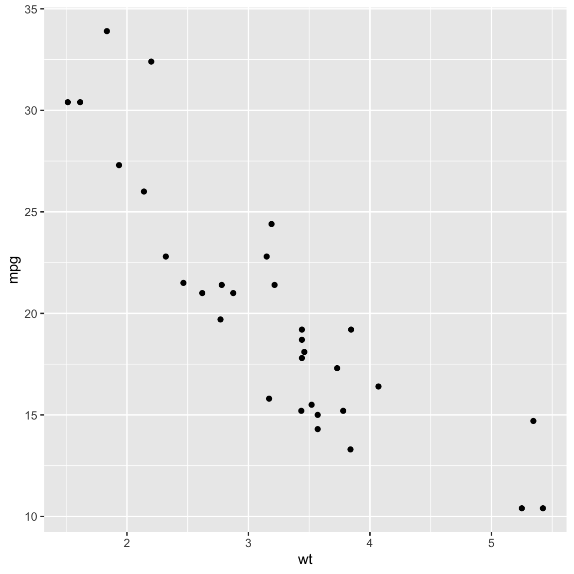
  geom_point()

• The pipe symbol (|>) is function composition.
  • f(g(x)) can be written x |> g |> f.
• aes is a function to define aesthetic associations between features of your plot and variables in the dataset.
• Parts of a ggplot are added togther with +
• The kind of plot is called its geometry.
  • geom_point makes a scatterplot.

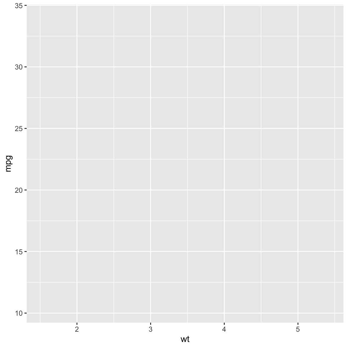
What if you forget … ?

mtcars |>
  ggplot(aes(x = wt,
             y = mpg))

Try “forgetting” other parts of the code to see what goes wrong.

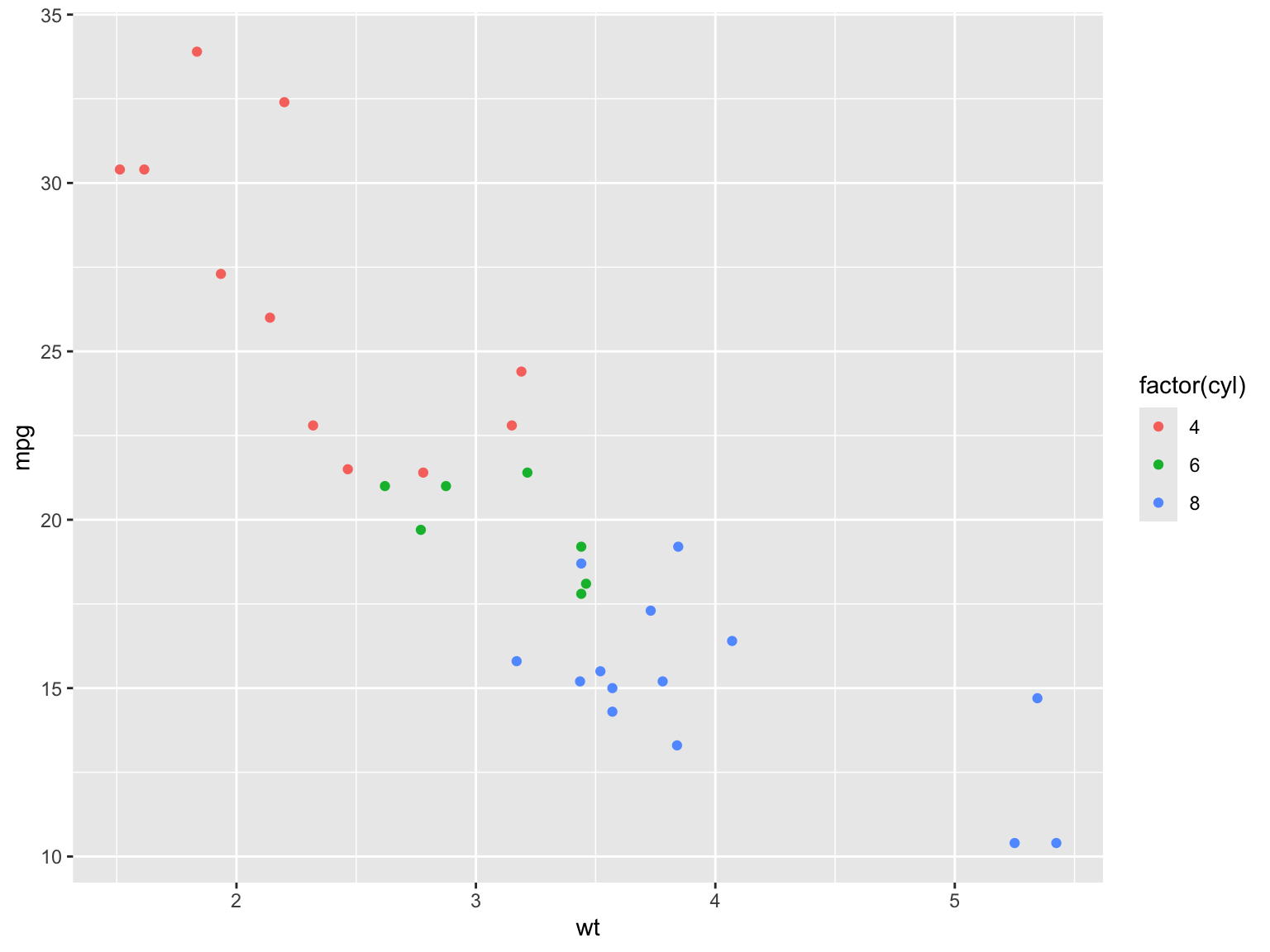
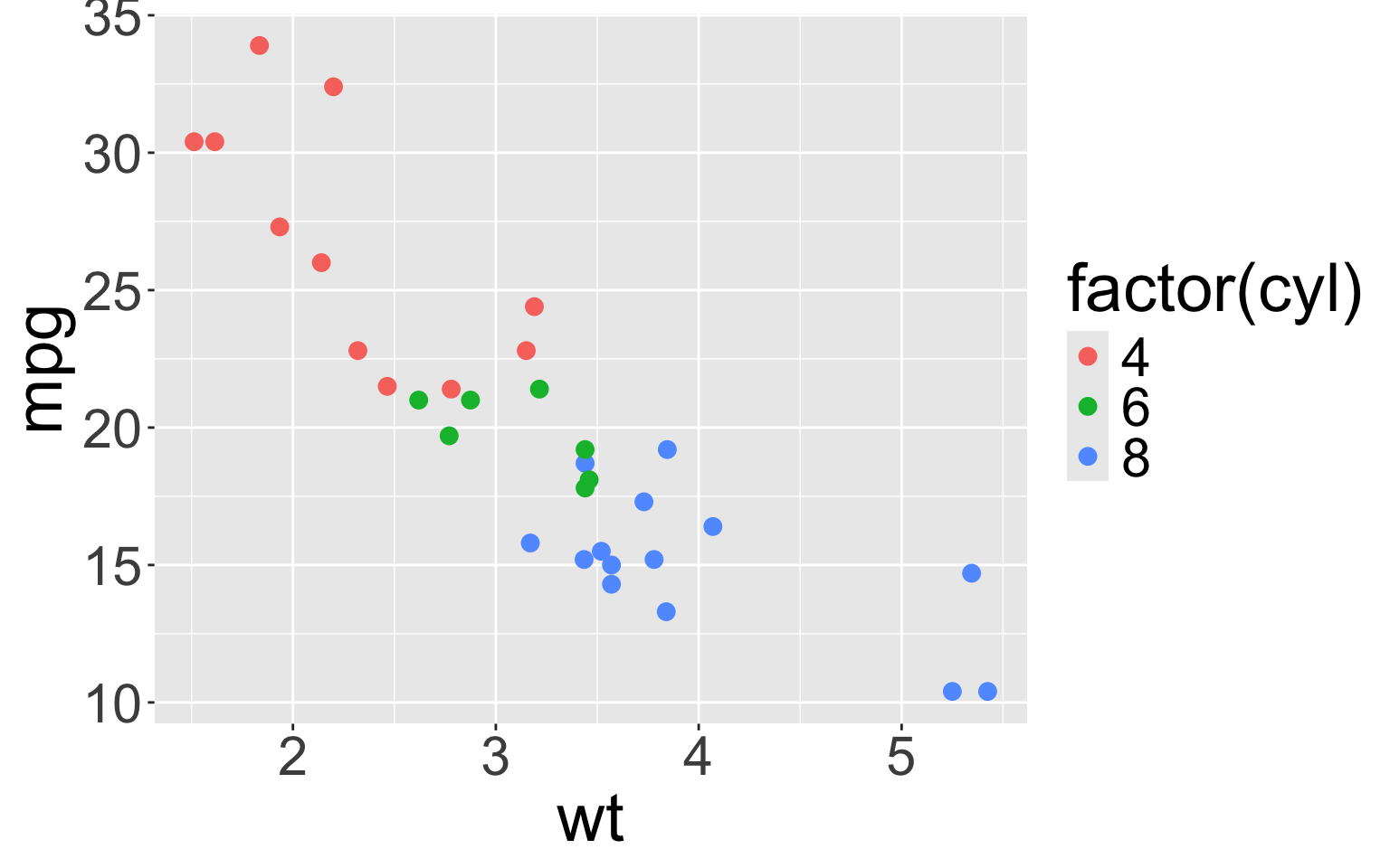
Add some colour

mtcars |>
  ggplot(aes(x = wt,
             y = mpg,
             color = factor(cyl))) + 
  geom_point()

cyl is a number, so I must turn it into a categorical variable (factor) to get a discrete colour scale.

Try using cyl instead of factor(cyl).

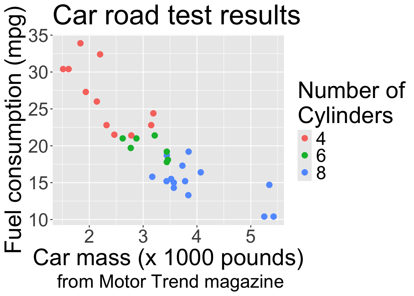
Make the text larger

mtcars |>
  ggplot(aes(x = wt,
             y = mpg,
             color = factor(cyl))) + 
  geom_point() +
  theme(text = element_text(size = 28))

Make the text larger

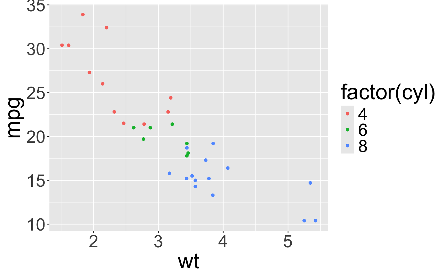
Make the symbols larger

mtcars |>
  ggplot(aes(x = wt,
             y = mpg,
             color = factor(cyl))) + 
  geom_point(size=3) + 
  theme(text = element_text(size = 28)) 

I’m setting the size of all the symbols, not connecting a variable to the size aesthetic. So don’t use aes.

geom_point (and any other geom) inherits the aesthetics from ggplot.

Make the symbols larger

Customize the labels

mtcars |>
  ggplot(aes(x = wt,
             y = mpg,
             color = factor(cyl))) + 
  geom_point(size=3) +
  theme(text = element_text(size = 28)) +
  labs(x = "Car mass (x 1000 pounds)", 
       y = "Fuel consumption (mpg)", 
       color = "Number of\nCylinders", 
       title = "Car road test results", 
       caption = "from Motor Trend magazine") 

Customize the labels

Summary

• Start with data

• Pipe (|>) into ggplot

• Define the aesthetics: aes(x = ..., y = ..., color = ..., shape = ...)

• Define the geometry: geom_point shown here, but there are lots more

• Customize text

Suggested reading

• Course notes: Making your first plot

• Healy. Section 2.6. Make your first figure

• R4DS. Chapter 3: Data visualization

• Lots more detail: The ggplot2 book

Exercises and Assignment

• Try these plotting commands on your own

• Assignment 1: Your first plotting exercises

Datasets to experiment with

• mtcars, iris and many other well-known data in datasets package
• penguins in palmerpenguins package
• gapminder in gapminder package (see Gapminder website too)
• diamonds in ggplot2 package

First steps with any dataset

Look at the data: use glimpse(mtcars) and View(mtcars) or just mtcars in the console.

Read documentation: ?mtcars or use search in the “Help” panel.

glimpse is in the dplyr package. Load it into your R session using library(tidyverse).